RelatedRates.mws

Related Rates

>    restart;

>   

Lesson Overview

The instantaneous rate of chage of a quantity is determined by a derivative. Likewise, when there is a relationship (equation) between several quantities, differentiation of the equation with respect to a variable yields a relationship involving the quantities and their rates of change. In the typical related rates problem, the original relationship and some combination of the quantities and their rates of change are provided. The objective is to determine one or more of the unknown quantities or rates of change. The keys to success in these problems are assembling the given information, identifying the variable to differentiate with respect to, correctly differentiating the original relationship, and - as the final step - solving for the unknown quantities.

The remainder of this lesson consists of examples illustrating the general approach used to solve almost any related rates problem. A customized maplet has been created for three of the four examples considered in this lesson. These maplets provide animations to help visualize the physical problem. These maplets can be used for other problems, including some of the homework problems. The RelatedRates  maplet [ Maplet Viewer][ MapleNet] helps to collect information and properly process the information in general related rate problems.

REQUEST: maplet improvement

The RelatedRates  maplet is one that I wrote quickly last semester. I have not had a chance to complete it the way I would like. First, the interface needs to be refined and improved. There should be a better way to manage the "active equation"; I used the popup menus just to see how they worked. While it would be simple to output results in MathML, I like the ability to edit a result (e.g., to remove extraneous results from a solve command) and then make it active. Maybe it would be possible to show results in MathML and have a "scratch work" area where command formatted expressions could be edited. Menus need to be created, particularly for Help. Let me know if you have any questions about this request.

>   

>   

Example 1

Problem

The volume of  a spherical balloon is increasing at a rate of 400 cubic inches per minute. Find the instantaneous rate at which the radius is increasing when the radius is 8 inches.

REQUEST: customized maplet

This maplet, RRSphere (?), would provide an interface to creating animations of an inflating balloon. A slider could be used to select the rate at which air is being added - or removed - from the balloon. The initial size/volume would be needed. Each frame would need to report the time, radius, volume, and possibly surface area. (Or, the user could select which of these quantities should be reported in each frame.) To be slightly more general, it would be nice to allow the user to specify if the given rate is volume, surface area, or radius. Let me know if you need any more information than this.

>   

Solution 1

Let the volume and radius of the spherical balloon be V  and r , respectively, and let t  denote time (the independent variable in this problem). The problem tells us that dV/dt  = 400 cubic inches/min and r = 8  inches. The objective is to determine dr/dt  when r = 8  inches and dV/dt = 400  inches/min.

No relationship between V  and r  is provided in the problem. However, because the balloon is a sphere, we know

>    q1 := V=4/3*Pi*r^3:
q1;

V = 4/3*Pi*r^3

Implicit in the problem is the statement that both volume and radius are functions of time, t . Thus, the relationship between V = V(t)  and r = r(t)  is really:

>    q2 := eval( q1, [V=V(t),r=r(t)] ):
q2;

V(t) = 4/3*Pi*r(t)^3

Differentiation of this relationship with respect to t  yields (by the Chain Rule):

>    q3 :=  diff( q2, t ):
q3;

diff(V(t),t) = 4*Pi*r(t)^2*diff(r(t),t)

Now that all differentiation is complete it is permissible to insert the given values and solve for the unknown quantity. Here, the given information is

>    d1 := [ diff(V(t),t)=400, r(t)=8 ]:
d1;

[diff(V(t),t) = 400, r(t) = 8]

and it is simple to solve for the rate of change of the radius

>    q4 := isolate( q3, diff(r(t),t) ):
q4;

diff(r(t),t) = 1/4*diff(V(t),t)/Pi/r(t)^2

When this numeric data is substituted into the differentiated relationship

>    q5 := lhs(q4) = eval( rhs(q4), d1 ):
q5;
`                         ` = evalf(rhs(q5));

diff(r(t),t) = 25/16/Pi

`                         ` = .4973591970

When the volume is increasing at 400 cubic inches per minute and the radius is 8 inches, the radius is increasing at a rate of 0.497 inches per minute.

>   

Solution 2 -- RelatedRates  Maplet

The solution of this problem can also be obtained using the RelatedRates  maplet [ Maplet Viewer][ MapleNet].

>   

Step 0

Launch the RelatedRates  maplet using either the Maplet Viewer, if you have Maple 8 on your local computer, or via MapleNet, if you want to access Maple over the WWW.

>   

Step 1

Enter all given information about the problem:

  • Enter the formula for the volume of a sphere, V=4/3*Pi*r^3 , in the Equation or Relationship  field.
  • In the Dependent Variable(s)  field, enter V  and r  between the square brackets: [ V, r ]
  • Time is the independent variable; in the Independent Variable  field, enter t .
  • There are no constants (parameters that do not change at all during the problem); do not change the Constants  field: [ ]  
  • The information that the radius is 8 inches is specified by changing the Values of Variables field to [ r = 8 ]  
  • The only given rate of change is dV/dt = 400  in ``^3 /min; in the Values of Rates of Change  field, enter D(V) = 400  
    Note the notation used to indicate a rate of change. This is a special notation that is understood only within the
    RelatedRates  maplet.
  • The rate of change of the radius is the quantity that we seek to determine; the Quantity to be determined  field should contain D(r)  

>   

Step 2

To prepare to differentiate the volume formula, make the Equation  or Relationship  field active.

The active field should now be V = 4/3*Pi*r^3  

>   

Note: The ``Active Equation''

The maplet performs operations on the Active Equation/Relationship . To make the contents of a field ``active'', position the cursor over the field and click the right mouse button, select the second entry: Make Active .

>   

Step 3

Differentiate the volume formula with respect to time by clicking the Diff wrt indep var  button. The result of this differentiation is displayed using D(V)  and D(r)  to represent the rates of change of volume and radius, respectively. Conclude by making this result the active equation.

The active equation should now be D(V) = 4*Pi*r^2*D(r)  

>   

Step 4

To substitute the given values and rates into the differentiated relationship, click on the Subs variables  button, make the result active, click on the Subs rates of change  button, and make this result active. (The two substitutions can be done in either order.)

At the end of Step 4 the active equation should be 400 = 256*Pi*D(r)  

>   

Step 5

Solve for the unknown quantity by clicking on the Solve for unknown quantity  button.

(To see a floating-point version of any result, click the right mouse button over a field, select the first menu option ( Manipulate ), and then evalf .)

The result should be D(r) = 25/16/Pi  or D(r) = .4973591970  

>   

This completes the solution using the RelatedRates  maplet. For this problem the maplet is not truly necessary. But, when there are more variables, a more complicated relationship, or other complicating features, the maplet can be a real timesaver.

>   

Example 2

Problem

An airplane flying north at v[1] = 1000  km per hour passes over your house at noon. An hour later a plane flying at v[2] = 800  km per hour changes trajectory to due east as it passes over your house. (Assume the planes fly on these trajectories forever.)

(i) Find the rate at which the distance between the planes is changing at 3 p.m..

(ii) Find the rate at which the distance between the planes is changing for any time after 1 p.m.. (Why does this answer not apply to times before 1 p.m.?)

(iii) Describe the rate at which the distance between the planes changes a long time after passing over your house.

>   

REQUEST: customized maplet

This maplet, RRPlanes(?), would provide an interface to creating animations of the two airplanes. The user would specify the direction and velocity of the two airplanes and the delay between the times they pass overhead. (It would certainly be simplest if the directions were perpendicular or parallel, but other orientations should be possible with a little trigonometry.) Each frame of the animation would report the time (in hours and minutes?) and the distance between the airplanes. Slider could be used to select the velocities of the two airplanes. (A large dot would be a suitable icon for each plane, but it should not be much more difficult to make the icons look like airplanes.)

>   

Solution

The fundamental relationship in this problem is the distance between the airplanes at any time after 1 p.m.. Let t = 0  correspond to 1 p.m.. Define a coordinate system in which your house is at the origin, due north is the positive y -axis, and due east is the positive x -axis. Then, for any time t  > 0, the positions of the two airplanes are (0, y ) and ( x ,0), respectively, where y = y(t)  and x = x(t)  are the distances of the two planes from your house. Thus,

  s^2 = x^2+y^2   or   s = sqrt(x^2+y^2)  

Moreover, dx/dt = 1000  km/hr and dy/dt = 800  km/hr.

The quantities s , x , and y  are all functions of t . In the RelatedRates  maplet, enter either of the above relationships between x , y , and s  and the dependent and independent variables. Differentiation of the distance relationship yields

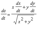
  2*s*ds/dt = 2*x*dx/dt+2*y*dy/dt         or         ds/dt = (x*dx/dt+y*dy/dt)/sqrt(x^2+y^2)  

(Take a minute to convince yourself that these are equivalent.)

Entering the given rate information in the maplet and substituting these values into either of the differentiated distance formulas leads to

  2*s*ds/dt = 2000*x+1600*y         or         ds/dt = (1000*x+800*y)/sqrt(x^2+y^2)  

Solving the first of these for ds/dt yields a convenient way to summarize both results:

  ds/dt = (1000*x+800*y)/s  

>   

(i)

At 3 p.m., t = 2 , the first plane has traveled x = 1000*(1+2)  = 3000 km beyond your house (remember that this plane passes over  your house an hour earlier than the second plane) while the slower airplane has traveled only y = 800*2  = 1600 km. Their separation at this time is s = sqrt(x^2+y^2)  = sqrt(3000^2+1600^2)  = 3400 km. Substituting these values in the formula for the rate of change of the distance yields:

  ds/dt = (1000*3000+800*1600)/3400  = 21400/17  = 1258.824 km/hr.

>   

(ii)

For a time after 1 p.m., t > 0, the first planes has traveled x = 1000*(1+t)  km beyond your house while the later airplane has traveled y = 800*t  km beyond your house. Thus,

  s = sqrt(x^2+y^2) = 200*sqrt(25+50*t+41*t^2)   and   ds/dt = 200*(25+41*t)/sqrt(25+50*t+41*t^2)  

To confirm this result, note that these formula with t = 2  produce the results in (a) and that ds/dt  could have been obtained by differentiating the distance formula expressed explicitly in terms of t .

These formula are not applicable for time before 1 p.m. ( t  < 0) because we do not know the trajectory of the second plane for times prior to 1 p.m..

>   

(iii)

The general formula for the rate of change of the separation between the two planes, as a function of t, was found in (b):

   ds/dt = 200*(25+41*t)/sqrt(25+50*t+41*t^2)  

>    q1 := 200*(25+41*t)/sqrt( 25 +50*t+41*t^2 ):
plot( q1, t=0..10, '`ds/dt`'=0..1500 );

[Maple Plot]

From this plot it is obvious that the instantaneous rate of change of the separation approaches a constant rather quickly. The precise value of this horizontal asymptote is

>    q2 := Limit( q1, t=infinity ):
q2 = value( q2 );
`` = evalf( q2 );

Limit(200*(25+41*t)/(25+50*t+41*t^2)^(1/2),t = infinity) = 200*41^(1/2)

`` = 1280.624847

>   

Example 3

Problem

Water drains from a spherical tank with a 20 foot radius at a rate of 2000 cubic foot per hour.

(i) Assuming the tank was full at noon, find the heights when 25%, 50%, 75%, and 100% of the water has drained from the tank.

(ii) What is the rate at which the water height in the tank is decreasing when half of the water has been drained?

>   

Hint: Volume of a Segment of a Sphere

The volume of a segment of a sphere with radius r  filled to height h  is

  V = Pi*h^2*(r-h/3) .

REQUEST: customized maplet

This maplet, RRTank(?), would provide an interface to creating animations of the draining of the tank. Ideally, the user would be able to select the shape of the tank from a list (circular cylinder, square cylinder, hemisphere (bottom), hemisphere (top), sphere, cone), the parameters for the selected tank, and either the rate at which water is drained from the tank or the rate at which the water height changes. (If a rate is negative, the user could specify the initial volume or height, or it could be assumed that the tank is full.) Each frame of the animation should display the time, height, volume, and rates of change for the height and volume.

I know a constant rate of change for the water height is not very realistic, but that would be made apparent by the animation.

>   

Solution

(i)

This part of the problem does not involve related rates, only algebra. Let noon be denoted with t = 0 . The tank is full when h = r ; the initial volume in the tank is

>    v := Pi*h^2*(r-h/3):
v0 := eval( v, h=r );

v0 := 2/3*Pi*r^3

A quarter of the volume has been drained from the tank when

>    q1 := v = 3/4*v0:
q1;

Pi*h^2*(r-1/3*h) = 1/2*Pi*r^3

There are three solutions to this equation

>    q2 := [solve( q1, {h} )];

q2 := [{h = (1/2*(2+2*I*15^(1/2))^(1/3)+2/(2+2*I*15^(1/2))^(1/3)+1)*r}, {h = (-1/4*(2+2*I*15^(1/2))^(1/3)-1/((2+2*I*15^(1/2))^(1/3))+1+1/2*I*3^(1/2)*(1/2*(2+2*I*15^(1/2))^(1/3)-2/(2+2*I*15^(1/2))^(1/3)...

All three solutions are real-valued

>    q3 := map( evalf@evalc, q2 );

q3 := [{h = 2.810037929*r}, {h = -.6417835274*r}, {h = .8317455986*r}]

and only one of them has 0 < h  < r:

>    q4 := op(op(select( s->evalb( rhs(op(s))/r>=0 and rhs(op(s))/r<=1 ), q3 ))):
q4;

h = .8317455986*r

With r = 20 , this translates into

>    eval( q4, r=20 );

h = 16.63491197

>   

Repeating these calculations to find the height when the tank is half empty

>    q5 := v = 1/2*v0:
q5;

Pi*h^2*(r-1/3*h) = 1/3*Pi*r^3

There are three solutions to this equation

>    q6 := [solve( q5, {h} )];

q6 := [{h = (1/2*(4+4*I*3^(1/2))^(1/3)+2/(4+4*I*3^(1/2))^(1/3)+1)*r}, {h = (-1/4*(4+4*I*3^(1/2))^(1/3)-1/((4+4*I*3^(1/2))^(1/3))+1+1/2*I*3^(1/2)*(1/2*(4+4*I*3^(1/2))^(1/3)-2/(4+4*I*3^(1/2))^(1/3)))*r},...

All three solutions are real-valued

>    q7 := map( fnormal@evalf@evalc, q6 );

q7 := [{h = 2.879385242*r}, {h = -.5320888864*r}, {h = .6527036446*r}]

and only one of them has 0 < h < r:

>    q8 := op(op(select( s->evalb( rhs(op(s))/r>=0 and rhs(op(s))/r<=1 ), q7 ))):
q8;

h = .6527036446*r

With r = 20 , this translates into

>    eval( q8, r=20 );

h = 13.05407289

>   

Repeating these calculations to find the height when the tank contains one quarter of its capacity:

>    q9 := v = 1/4*v0:
q9;

Pi*h^2*(r-1/3*h) = 1/6*Pi*r^3

There are three solutions to this equation

>    q10 := [solve( q9, {h} )];

q10 := [{h = (1/2*(6+2*I*7^(1/2))^(1/3)+2/(6+2*I*7^(1/2))^(1/3)+1)*r}, {h = (-1/4*(6+2*I*7^(1/2))^(1/3)-1/((6+2*I*7^(1/2))^(1/3))+1+1/2*I*3^(1/2)*(1/2*(6+2*I*7^(1/2))^(1/3)-2/(6+2*I*7^(1/2))^(1/3)))*r}...

All three solutions are real-valued

>    q11 := map( evalf@evalc, q10 );

q11 := [{h = 2.942241851*r}, {h = -.3843671529*r}, {h = .4421253017*r}]

and only one of them has 0 < h  < r :

>    q12 := op(op(select( s->evalb( rhs(op(s))/r>=0 and rhs(op(s))/r<=1 ), fnormal(q11) ))):
q12;

h = .4421253017*r

With r = 20 , this translates into

>    eval( q12, r=20 );

h = 8.842506034

>   

(ii)

The fundamental relationship for this problem is the volume formula for a segment of a sphere with radius r  filled to height h :

  V = Pi*h^2*(r-h/3)  

where r is a constant (r=20 ft) and V and h are functions of the independent variable, t. Enter the volume formula, variable information, value of the constant, and the given rate of change  in the RelatedRates  maplet. The derivative of the volume formula is

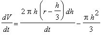
  dV/dt = 2*Pi*h*(r-h/3)*dh/dt-Pi*h^2/3   dh/dt  

That is,

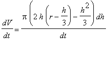
  dV/dt = Pi*(2*h*(r-h/3)-h^2/3)*dh/dt  = Pi*h*(2*r-h)*dh/dt  

Therefore, in general,

>    q13 := Diff(h,t) = 1/(Pi*h*(2*r-h))*Diff(V,t):
q13;

Diff(h,t) = 1/Pi/h/(2*r-h)*Diff(V,t)

Inserting the known values:

>    data := [ Diff(V,t)=-2000, r=20, eval(q8,r=20) ]:
data;

[Diff(V,t) = -2000, r = 20, h = 13.05407289]

yields

>    lhs(q13) = evalf( eval( rhs(q13), data ) );

Diff(h,t) = -1.809843235

The water height is decreasing at a rate of 1.81 ft/hr.

>   

Example 4

Problem

A (spherical) snowball melts at a rate proportional to its surface area.

(i) Show that its radius shrinks at a constant rate.

(ii) If, during the first hour, half of the snowball melts, how long will it take to melt completely?

>   

REQUEST: customized maplet -- NOT!

I do not see a need for a customized maplet for this problem.

>   

Solution

(i)

The volume, V, and surface area, S, for a sphere of radius r are

>    v := 4/3*Pi*r^3:
V = v;

V = 4/3*Pi*r^3

>    s := 4*Pi*r^2:
S = s;

S = 4*Pi*r^2

Assuming the radius changes with time, the volume and surface area will be functions of time.

>    q1 := eval( V=v, [V=V(t),r=r(t)] ):
q1;

V(t) = 4/3*Pi*r(t)^3

>    q2 := eval( S=s, [S=S(t),r=r(t)] ):
q2;

S(t) = 4*Pi*r(t)^2

The rate of change of the volume is

>    q3 := diff( q1, t ):
q3;

diff(V(t),t) = 4*Pi*r(t)^2*diff(r(t),t)

Note the presence of the surface area, S(t) = 4*Pi*r(t)^2 , in this formula. This allows us to rewrite the rate of change of the volume as

>    q4 := lhs(q3) = S(t)*diff( r(t),t ):
q4;

diff(V(t),t) = S(t)*diff(r(t),t)

If the volume changes at a rate proportional to the surface area, then dV/dt = k*S , for some constant k . From the above equation it is seen that

  dr/dt = k ,

i.e., the radius changes at a constant rate.

>   

(ii)

We know the radius decreases at a constant, but currently unknown, rate. If we call the rate k , then

>    q1 := r = r0 - k*t:
q1;

r = r0-k*t

The snowball disappears when r = 0 :

>    q2 := isolate( eval(q1,r=0), t );

q2 := t = r0/k

The information that half the snowball melts in the first hour is used to determine r0/k . First, if half of the snowball melts in the first hour, then

>    q3 := eval( v, eval(q1,t=1) ) = 1/2*(4/3*Pi*r0^3);

q3 := 4/3*Pi*(r0-k)^3 = 2/3*Pi*r0^3

This equation can be solved for r0  in terms of k  

>    q4 := solve( q3, {r0} );

q4 := {r0 = (2^(2/3)+2^(1/3)+2)*k}, {r0 = (-1/2*2^(2/3)-1/2*2^(1/3)+2+1/2*I*3^(1/2)*(2^(2/3)-2^(1/3)))*k}, {r0 = (-1/2*2^(2/3)-1/2*2^(1/3)+2-1/2*I*3^(1/2)*(2^(2/3)-2^(1/3)))*k}

Only real-valued solutions are of interest, so all solutions containing I  must be removed:

>    q5 := op(remove( has, [q4], I ));

q5 := {r0 = (2^(2/3)+2^(1/3)+2)*k}

When this is substituted into the formula for the time when the snowball disappears we find that the snowball disappears when

>    q6 := eval( q2, q5 ):
q6;
`` = evalf(rhs(q6));

t = 2^(2/3)+2^(1/3)+2

`` = 4.847322102

That is, in about 4 hours, 50 minutes, the snowball is completely melted.

>   

Lesson Summary

Related rate problems can be difficult even though they generally involve only algebra, sometimes geometry, and the differentiation rules - particularly the chain rule. The most difficult part of the problem can be identifying the quantities that change and the fundamental relationship between the varying quantities. The most common errors are

Be alert to these potential pitfalls!

The four examples in this lesson provide a good framework for solving related rate problems with or without the RelatedRates  maplet [ Maplet Viewer][ MapleNet].

>   

What's Next?

The online and textbook homework assignments should be completed with or without the RelatedRates  maplet [ Maplet Viewer][ MapleNet]. Be sure to work enough practice problems before attempting the online homework assignment and textbook homework assignment.

The Global Analysis, Local Analysis, Optimization Problems, and Graphing lessons provide a complete discussion of the use of calculus for locating and classifying the most interesting point on the graph of a function. The Mean Value Theorem lesson is an obvious but important theoretical result that, like the Intermediate Value Theorem, is also used in a variety of applications.

>   

>   

>