Example 1
Show that among all rectangles with a fixed perimeter, the square has the maximum area.
| > |
Solution
The first phrase provides a constraint for this problem. Denote the perimeter by
![]() and let
and let
![]() and
and
![]() denote the length and width of the rectangle, respectively. Then,
denote the length and width of the rectangle, respectively. Then,
| > | Con := 2*L+2*W=P: Con; |
![]()
Implicit in this problem are the geometric constraints that
![]() and
and
![]() are not negative:
are not negative:
| > | Con2 := L >= 0: Con3 := W >= 0: Con2, Con3; |
![]()
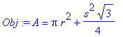
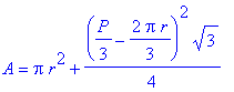
Since area,
![]() , is the quantity to be maximized, the objective function is
, is the quantity to be maximized, the objective function is
| > | Obj := A = L*W: Obj; |
![]()
The initial formulation of this problem as an optimization problem is
| > | PrintOptProb(max,Obj,Con,Con2,Con3); |
max A = L*W
s.t. 2*L+2*W = P
0 <= L
0 <= W
where s.t. is an abbreviation for "subject to".
| > |
The next step is to reformulate the problem with an objective function depending on only one variable and the constraint expressed as an appropriate interval. The perimeter constraint can be used to find an expression for either
![]() or
or
![]() in terms of the other variable (and the parameter
in terms of the other variable (and the parameter
![]() ):
):
| > | Sub := isolate( Con, L ): Sub; |
![]()
The objective function, expressed in terms of the variable
![]() , is
, is
| > | Obj1 := eval( Obj, Sub ): Obj1; |
![]()
The nonnegativity of
![]() provides one endpoint for the interval. The nonnegativity of
provides one endpoint for the interval. The nonnegativity of
![]() must yield the other endpoint. In fact, using the substitution identified above, the constraint for
must yield the other endpoint. In fact, using the substitution identified above, the constraint for
![]() can be written as
can be written as
| > | q1 := eval( Con2, Sub ): q1; |
![]()
or, solving for
![]() ,
,
| > | Con4 := isolate( q1, W ): Con4; |
![]()
The resulting optimization problem is
| > | PrintOptProb( max, Obj1, Con3, Con4 ); |
max A = (1/2*P-W)*W
s.t. 0 <= W
W <= 1/2*P
Because this problem is asking for the global maximum of a continuous function on a closed and bounded interval, we know the maximum value will occur at a critical point of the objective function in the interval. The endpoints are
| > | EndPt := 0, P/2: EndPt; |
![]()
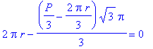
Stationary points occur when the derivative of the objective function is zero
| > | dObj1 := diff( rhs(Obj1), W ); StatPtEqn := dObj1 = 0: StatPtEqn; |
![]()
![]()
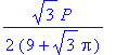
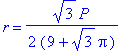
The one stationary point is
| > | StatPt := solve( StatPtEqn, W ): StatPt; |
![]()
(Note that this is in the interval, in fact, it is the midpont of the interval.) And, there are no singular points
| > | SingPt := NULL: |
Now, evaluating the objective function at each critical point yields
| > | seq( ['W'=W,Obj1], W=[EndPt,StatPt,SingPt] ); |
![[W = 0, A = 0], [W = 1/2*P, A = 0], [W = 1/4*P, A = 1/16*P^2]](images/Optimization26.gif)
From this list it is quite clear that the maximum area,
 , occurs when
 , i.e., at the stationary point.
While we have found the global maximum on this interval, we are not done. It still remains to verify that the resulting rectangle is a square. This will be done by showing that
![]() for the optimal width:
for the optimal width:
| > | q2 := eval( Sub, W=StatPt ): W=StatPt; q2; |
![]()
![]()
Observation:
Notice that if the geometric constraints had been formulated as strict inequalities,
![]() > 0 and
> 0 and
![]() > 0, then the interval expressed solely in terms of
> 0, then the interval expressed solely in terms of
![]() would be the open interval: 0 <
would be the open interval: 0 <
![]() <
<
![]() . In this case the argument that the critical point is the global maximum would require consideration of appropriate one-sided limits. It is generally much easier to simply allow the degenerate geometric objects that correspond to the endpoints and work with a closed and bounded interval. Sometimes these endpoints do, in fact, yield the desired optimal configuration.
. In this case the argument that the critical point is the global maximum would require consideration of appropriate one-sided limits. It is generally much easier to simply allow the degenerate geometric objects that correspond to the endpoints and work with a closed and bounded interval. Sometimes these endpoints do, in fact, yield the desired optimal configuration.
| > |

![[Maple Plot]](images/Optimization91.gif)
![A[tri] = 1/4*s^2*3^(1/2)](images/Optimization144.gif)
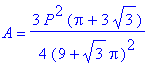
![q2 := [r = 0, s = 1/3*P, A = 1/36*P^2*3^(1/2)], [r = 1/2*P/Pi, s = 0, A = 1/4/Pi*P^2], [r = 1/2*3^(1/2)*P/(9+3^(1/2)*Pi), s = 3*P/(9+3^(1/2)*Pi), A = 3/4*P^2*(Pi+3*3^(1/2))/(9+3^(1/2)*Pi)^2]](images/Optimization163.gif)
![q2 := [r = 0, s = 1/3*P, A = 1/36*P^2*3^(1/2)], [r = 1/2*P/Pi, s = 0, A = 1/4/Pi*P^2], [r = 1/2*3^(1/2)*P/(9+3^(1/2)*Pi), s = 3*P/(9+3^(1/2)*Pi), A = 3/4*P^2*(Pi+3*3^(1/2))/(9+3^(1/2)*Pi)^2]](images/Optimization164.gif)


![L[1] = c*S[1]/d[1]^2](images/Optimization186.gif)
![L[2] = c*k*S[1]/d[2]^2](images/Optimization187.gif)
![Obj := c*S[1]/d[1]^2+c*k*S[1]/d[2]^2](images/Optimization188.gif)
![Obj1 := c*S[1]/d[1]^2+c*k*S[1]/(10-d[1])^2](images/Optimization197.gif)
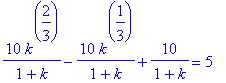
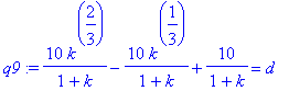
![d[1] = 10/(1+k)*k^(2/3)-10*k^(1/3)/(1+k)+10/(1+k)](images/Optimization200.gif)
![d2Obj1 := 6*c*S[1]*(10000-4000*d[1]+600*d[1]^2-40*d[1]^3+d[1]^4+k*d[1]^4)/d[1]^4/(-10+d[1])^4](images/Optimization201.gif)
![-3/5000*(1+k)^5*k*(-k^2+3*k^(5/3)-6*k^(4/3)+7*k-6*k^(2/3)+3*k^(1/3)-1)*c*S[1]/(-k+k^(2/3)-k^(1/3))^4/(k^(2/3)-k^(1/3)+1)^4](images/Optimization202.gif)
![Limit(c*S[1]/d[1]^2+c*k*S[1]/(10-d[1])^2,d[1] = 0,right) = infinity](images/Optimization204.gif)
![Limit(c*S[1]/d[1]^2+c*k*S[1]/(10-d[1])^2,d[1] = 10,left) = infinity](images/Optimization205.gif)
![d[1] = 10/(1+k)*k^(2/3)-10*k^(1/3)/(1+k)+10/(1+k)](images/Optimization208.gif)
![[Maple Plot]](images/Optimization219.gif)