DerivTrig.mws
Derivatives of Trigonometric Functions
Auxiliary Procedures
| > |
DerivativeTable := proc( f, x, orders )
local n, T;
n := nops(orders);
T := Matrix( n, 2, (i,j)->`if`(j=1,orders[i],diff(f,x$orders[i])) );
return T
end proc:
|
Lesson Overview
We now have all the tools necessary to differentiate trigonometric functions. The fundamental trigonometric functions are sine and cosine. Once the derivatives of these are known, the derivatives of tangent, secant, cotangent, and cosecant can be obtained with the Quotient, Power, and
Chain Rules. Thus, our primary objective is to find the derivative of sine and cosine. This will be done via the definition and will involve the two special limits from the
Limits of Trigonometric Functions lesson. Additional examples will provide additional practice with all of the
Derivative Rules, including the
Chain Rule.
The
DerivativePlot
maplet [
Maplet Viewer][
MapleNet] is introduced as a useful tool for creating a plot of a function and one or more of its derivatives. The
Differentiation
maplet [
Maplet Viewer] [
MapleNet] continues to be a useful tool for practicing the use of the
Differentiation Rules. But, do not become dependent upon these maplets --- be sure you can find derivatives by hand!
Derivatives of the Sine and Cosine Functions
Graphs of the sine and cosine functions are continuous and have a tangent line at all points. This means the sine and cosine functions should be differentiable everywhere.
To form a picture of the derivative of the sine function, use the
DerivativePlot
maplet [
Maplet Viewer][
MapleNet]. Launch this maplet, then set the
Function
to be
sin(x)
,
a
=
-2*Pi
,
b=
2*Pi
, and
orders=
1
then click
Plot
. The graph of the derivative of the sine function looks familiar --- with a period of
 , amplitude 1 with a maximum at
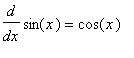
 it looks like the cosine function. This leads to the conjecture:
Now, change the
Function
to
cos(x)
and click
Plot
. The derivative of cosine has period
 , amplitude 1 with a zero at
 and a minimum around
 and another zero around
 ; this sounds like the negative of the cosine function. Based on this we conjecture:
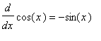
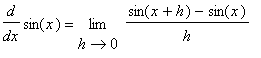
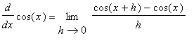
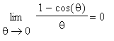
To determine if these conjectures are correct, turn to the definition of the derivative:
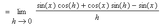
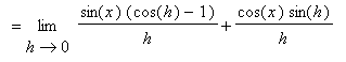
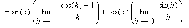
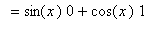

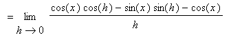

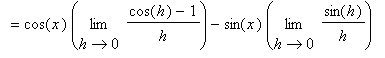
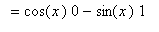

You should now understand why we spent so much time in the
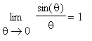
Limits of Trigonometric Functions lesson looking at the two special limits:
 and
and
Because of the way the derivatives of sine and cosine are related it should be interesting to look at the higher-order derivatives of these functions.
| > |
DerivativeTable( sin(x), x, [$1..8] ),
DerivativeTable( cos(x), x, [$1..8] );
|
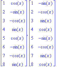
Thus, higher-order derivatives of sine and cosine are cyclic (with period 4).
Derivatives of Other Trigonometric Functions
The derivatives of the sine and cosine function together with the Quotient, Power, and
Chain Rules are all that is needed to discover the derivatives of tangent, secant, cotangent, and cosecant.
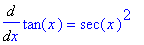
First, for the tangent function:
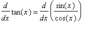
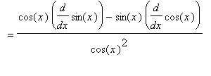

 .
.
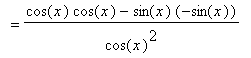
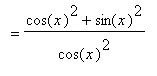
The derivative of the secant function can be found with the Power and Chain Rules:
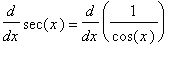
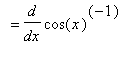
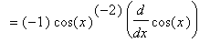
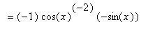


Note the use of the
Chain Rule in this derivation.
The derivatives of the cotangent and cosecant functions can be similarly derived.
All six trigonometric derivatives are summarized in the table below.
![MATRIX([[diff(sin(x),x) = cos(x), diff(cos(x),x) = -sin(x)], [diff(tan(x),x) = sec(x)^2, diff(cot(x),x) = -csc(x)^2], [diff(sec(x),x) = sec(x)*tan(x), diff(csc(x),x) = -csc(x)*cot(x)]])](images/DerivTrig38.gif)
A comparison of the entries in the first column with the corresponding entry in the second column of the table reveals a relationship between the derivatives of a trigonometric function and its ``co'' function:
change the sign and change all functions to their co-function.
For this reason it is not essential that you memorize the derivatives of cotangent and cosecant.
Examples
You are strongly encouraged to use the
Differentiation
maplet [
Maplet Viewer] [
MapleNet] to follow each step of the differentiation in each example.
Example 1:
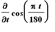
This derivative is computed using the
Chain Rule:
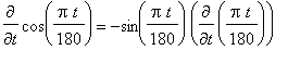
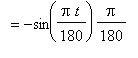


Confirmation of this result with Maple is obtained as follows:
| > |
f1 := cos( Pi*t/180 ):
df1 := Diff( f1, t ):
df1 = value( df1 );
|
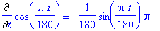
The factor
 in this function converts an angle from degrees to radians. This result shows that this factor also relates the rate of change of the cosine of an angle measured in radians to the rate of change of the cosine of an angle measured in degrees.
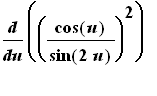
Example 2:
To simplify this answer further use the double angle formulae:
 and
and
 .
.
These yield
Further simplifications are possible with another application of the double angle formula for sine:
In hindsight, note that the function to be differentiated can be simplified using the double angle formula for sine.


Use the
Differentiation
maplet [
Maplet Viewer] [
MapleNet] to verify the derivative of this expression agrees with the previous results of this example.
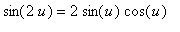
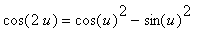
To use Maple to confirm the manual computations above it will be necessary to explicitly tell Maple which trigonometric identities to use at various points along the way. We begin by entering these identities:
| > |
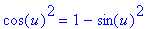
id1 := u->cos(u)^2=1-sin(u)^2:
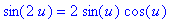
id2 := u->sin(2*u)=2*sin(u)*cos(u):
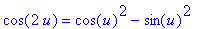
id3 := u->cos(2*u)=cos(u)^2-sin(u)^2:
id1(u);
id2(u);
id3(u);
|
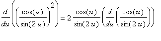
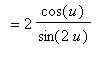
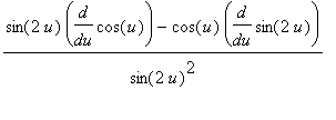
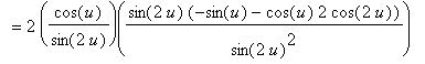
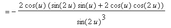
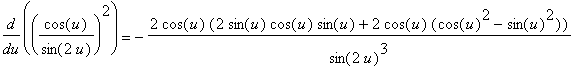
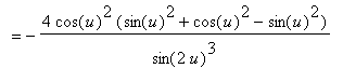
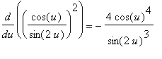
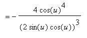
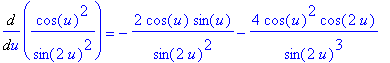
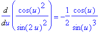
The derivative of the function in its original form is
| > |
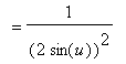
f2 := ( cos(u)/sin(2*u) )^2:
df2a := Diff( f2, u ):
df2a = value( df2a );
|
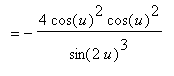
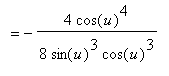
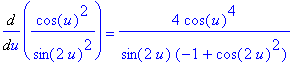
Combining the two terms on right-hand side yields
| > |
df2b := simplify( value(df2a) ):
df2a = df2b;
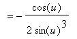
|
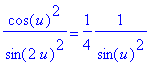
Maple's result takes this form because Maple ``simplified''
 to
to
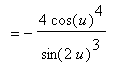
 . To undo this step, use Maple's
simplify
command with a
side relation
. The result is
. To undo this step, use Maple's
simplify
command with a
side relation
. The result is
| > |
df2c := simplify( df2b, [id1(u)] ):
df2a = df2c;
|

Which agrees with the result obtained manually.
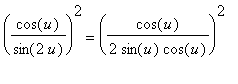
When the double angle formula for sine is applied to the function prior to differentiation:
| > |
f2a := simplify( f2, [id2(u)] ):
f2 = f2a;
|
and so
| > |
df2d := diff( f2a, u ):
df2a = df2d;
|
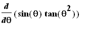
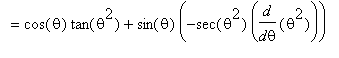
Example 3:
Note that the second term is
 , not
, not
 .
.
This derivative can be found using the Product and
Chain Rules:
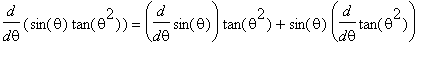
Computation of this derivative in Maple could be done as follows:
| > |
f3 := sin(theta)*tan(theta^2):
df3 := Diff( f3, theta ):
df3 = value( df3 );
|
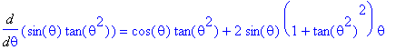
This answer differs from ours in appearance only. Note that Maple reports
| > |
q1 := Diff( tan(x), x ):
q1 = value( q1 );
|
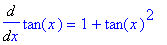
To force Maple to replace powers of tangent with secant we supply a fourth trigonometric identity:
| > |
id4 := u->tan(u)^2=sec(u)^2-1:
id4(x);
|
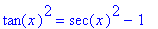
Then, supplying this identity to
simplify
as a
side relation
:
| > |
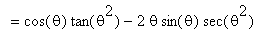
q1 = simplify( value(q1), [id4(x)] );
|
Applying this same approach to this example,
| > |
df3 = simplify( value(df3), [id4(theta^2)] );
|
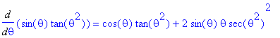
Except for the unfortunate separation of the terms in the
 factor, this is exactly our result.
Lesson Summary
The trigonometric functions are differentiable at all points in their domain. The derivatives of the fundamental functions are
![MATRIX([[diff(sin(x),x) = cos(x), diff(cos(x),x) = -sin(x)], [diff(tan(x),x) = sec(x)^2, diff(cot(x),x) = -csc(x)^2], [diff(sec(x),x) = sec(x)*tan(x), diff(csc(x),x) = -csc(x)*cot(x)]])](images/DerivTrig90.gif)
What's Next?
By now you should be very comfortable using the
Differentiation
maplet [
Maplet Viewer] [
MapleNet] to check your work. While this tool is useful and powerful, remember that you must also develop your manual skills. After correctly answering a few of the online practice problems, complete the
textbook homework assignment and the
online homework assignment.
In the
Implicit Differentiation lesson the Power Rule will be verified for all rational exponents and we will learn how to find the slope of the tangent line to any curve - not just the graph of a function. This will conclude the unit on differentiation.