DerivRules.mws
Differentiation Rules
Lesson Overview
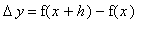
Evaluation of derivatives using the definition hinges on the ability to evaluate the limit of the difference quotient. This is tedious and time consuming. Even worse, the limits can be extremely difficult to evaluate. The Differentiation Rules are a collection of general rules for computing derivatives formed from polynomials, powers, roots, and constant multiples, sums, differences, products, quotients of these types of functions. Compositions of functions are handled separately, in the
Chain Rule lesson.
Be careful to not confuse the
Limit Laws and Differentiation Rules. While many are analogous, others are completely different.
The
Differentiation
maplet [
Maplet Viewer] [
MapleNet] provides an excellent tool to learn the names of the Differentiation Rules and how they can be applied to evaluate a derivative. The three examples provided in this worksheet should get you started using this tool.
The Differentiation Rules
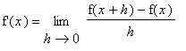
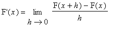
In general, derivatives can be evaluated by applying the definition as in Examples 1 - 3 in the
Precise Definition of the Derivative lesson. The first few rules are fairly simple, almost obvious. But, starting with the Product Rule, the rules are not so obvious and are quite different from the corresponding
Limit Laws.
Let f and g be functions that are differentiable at x and let k be a constant.
![MATRIX([[Name,
Formula, `Extra Conditions`], [___________________, ___________________________
__________________, ____________________________], [Constant, diff(k,x) = 0, non
e], [Identity, diff(x,x) = ...](../HTML-GIF/images/DerivRules1.gif)
Note the conditions listed in the third column. If the conditions for a rule are not satisfied, the rule cannot be used to justify the evaluation of a limit.
Proofs
It is very difficult to give a formal proof of the Differentiation Rules using Maple. In some cases it is possible to give a geometric argument, using a Maple-generated graph, in other cases Maple can be used to identify difference quotients as derivatives. But, care must be exercised to distinguish between a proof and an argument based on "because Maple says so".
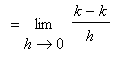
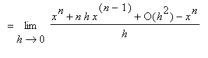
Proof of Constant Rule
The Constant Rule can be understood by noting that the graph of a constant function is a horizontal line, i.e., has slope 0.
| > |
plot( 2.3, x=-3..3, title="Constant functions have slope 0" );
|
![[Maple Plot]](images/DerivRules12.gif)
The defintion of the derivative of a constant function is simple to apply. Define the constant function:
 . Then apply the definition of the derivative and simplify:


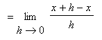
Proof of Identity Rule
The Identity Rule can be answered using our knowledge of linear functions. The graph of the function
 is the straight line through the origin with slope
 for all
 . Thus,
 .
.
A rigorous proof based on the definition is not difficult either:


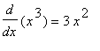
Proof of Power Rule (
 a positive integer)
First, note that the Power Rule with
 is the Identity Rule:
 =
=
 =
=
 = 1
= 1
We have also seen (Example 1 in the
Precise Definition of the Derivative lesson) that
 , that is the Power Rule holds for
 .
.
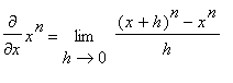
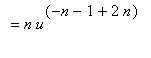
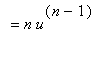
The proof of the Power Rule when
 is a positive integer is based on the patterns observed in
| > |
for i from 1 to 10 do
(x+h)^i = expand( (x+h)^i )
end do;
|

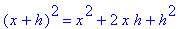
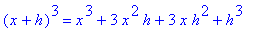


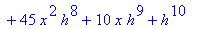
In particular, note that
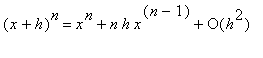 . (We say that
 when
when
 exists; in particular,
 means
means
 .) From here it is not difficult to obtain

The Power Rule does hold when the exponent is zero, a negative integer, a rational number, or an irrational number The case for
 is the Constant Rule. The proofs of the remaining cases depend on results that will come later in the course. The first of these, negative integers, is Example 4 in this lesson.
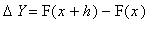
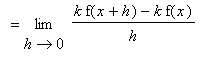
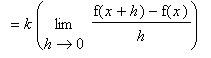
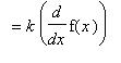
Proof of Constant Multiple Rule
The Constant Multiple Rule should be contemplated prior to proving. Let
 and
and
 be the run and rise for f. If
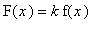 , then the rise for F will be
 =
=
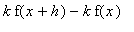 =
=
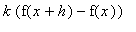 =
=
 .
.
Thus,
 for all
 > 0 and so
 =
=
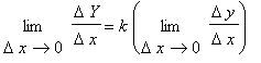 =
=

A rigorous proof based on the definition is not difficult either:
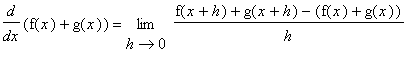
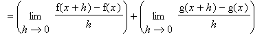
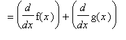
Proof of Sum Rule
The Sum Rule makes intuitive sense. The rate of change of the sum of two functions should be the sum of their rates of change:
To prove the Sum Rule it is necessary to work with f and g as arbitrary differentiable functions:
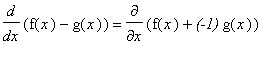
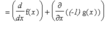
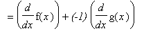
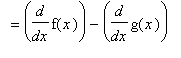
Proof of Difference Rule
A proof of the Difference Rule can be given in exactly the same form as for the Sum Rule. An alternative is to use both the Constant Multiple and Sum Rules:
To prove the Sum Rule it is necessary to work with f and g as arbitrary differentiable functions:
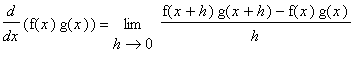
Proof of Product Rule
On first thought one might think the Product Rule should simply multiply the derivatives.
This is wrong!
A simple example illustrating this fallacy is
 with
with
 =
=
 . Then
 = 1 but
 =
=
 =
=
 .
.
The proof of the Product Rule requires a little extra work to put the difference quotient for the product in a form where derivatives of f and g can be identified. The key is to add and subtract the same quantity in the numerator so that difference quotients for f and g can be isolated in separate pairs of terms.
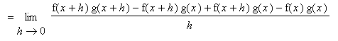
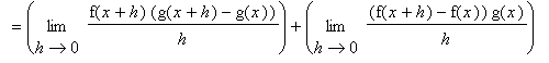
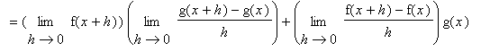
Note that
 because the assumption that f is differentiable at
 implies f is continuous at
 .
.
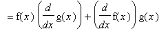
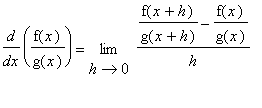
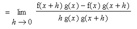
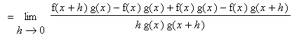
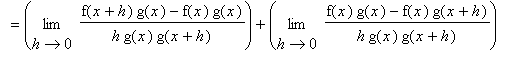
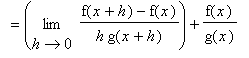
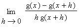
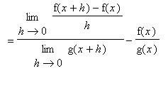
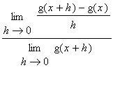
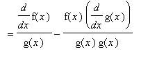
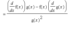
Proof of Quotient Rule
The proof of the Quotient Rule is similar to the proof of the Product Rule in that it involves the addition and subtraction of the same quantity from the difference quotient. This quantity is chosen so that difference quotients involving f and g can be identified.
Three Examples
The following three examples demonstrate the use of these derivatives in the evaluation of derivatives. Of the three, only the first example is even remotely reasonable to attempt to evaluate with the definition.
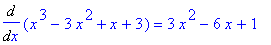
Example 1: Use the Differentiation Rules to evaluate
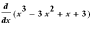
![MATRIX([[`Algebraic Manipulation`, Remarks], [________________________, ________________________], [diff(x^3-3*x^2+x+3,x), `original derivative`], [diff(x^3,x)-diff(3*x^2,x)+diff(x,x)+diff(3,x), `appli...](images/DerivRules107.gif)
That is,
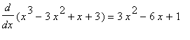 .
.
This result can be verified using Maple's
diff
(or
Diff
) command:
| > |
q1 := x^3-3*x^2+x+3:
Diff( q1, x ) = diff( q1, x );
|
In addition to following the steps provided in the examples you are encouraged to repeat these examples in the
Differentiation
maplet [
Maplet Viewer][
MapleNet]. To specify a problem in the
Differentiation
maplet note that the top line of this maplet contains fields for the function and variable. Press the
Start
button, then apply the rules of differentiation by clicking the corresponding button in the
Differentiation
maplet. The menu bars provide a summary of each known rule (
Rule Definition
),
help
, and another way to apply rules (
Apply the Rule
). Note that the selected rule is generally applied to the first possible occurrence in the expression; it may be necessary to apply a rule multiple times in succession. (This maplet does not have a Difference rule. Instead, as suggested by the proof, use the Sum and Constant Multiple rules.)
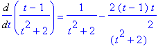
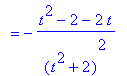
Example 2: Use the Differentiation Rules to evaluate
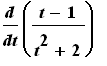
This derivative will be computed by first applying the Quotient Rule. The remaining derivatives require only the Sum, Difference, Constant, Identity, and Power Rules.
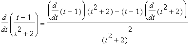
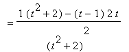
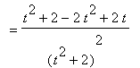
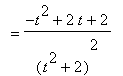
This derivative agrees with the one found by Maple:
| > |
q2 := (t-1)/(t^2+2):
Diff( q2, t ) = diff( q2, t );
`` = simplify( diff(q2,t) );
|
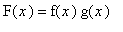
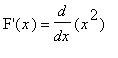
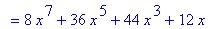
Example 3: Use the Differentiation Rules to evaluate
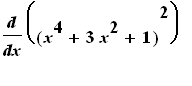
At first glance we do not (yet) have the necessary techniques to evaluate this derivative. But, once we note that this problem can be written as the product of (
x^4+3*x^2+1
) with itself, it is seen that the Product Rule can be used. (Note that the
Differentiation
maplet does not believe the Product Rule can be applied here. The hint suggests that the Chain Rule should be applied. Since we do not yet know the Chain Rule, you will have to follow this example without the use of the
Differentiation
maplet.)
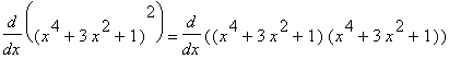
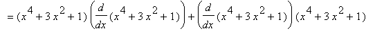
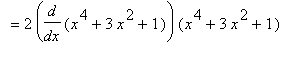
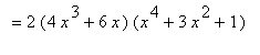
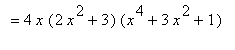
Note that an alternate approach to this problem is to compute
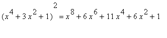
and so
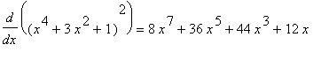
To cross-check these results, we turn to Maple to help with the algebra. First, the result using the Product Rule can be summarized as
| > |
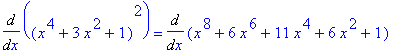
q3 := (x^4+3*x^2+1)^2:
Diff( q3, x ) = expand( diff(q3,x) );
|
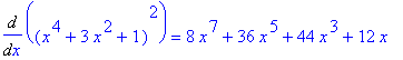
The derivative obtained when the function is expanded prior to being differentiated is
| > |
Diff( q3, x ) = Diff( expand(q3), x );
`` = diff( expand(q3), x );
|
This confirms our hand computations and verifies that the two approaches yield the same result.
Note that while expansion was easier for this problem, the Product Rule is easier to apply in most problems involving a power as in this example. An even more efficient method for computing the derivative of a composition of two functions will be addressed in the
Chain Rule lesson.
Extending the Power Rule to Negative Integer Exponents
The Quotient Rule can be applied to extend the Power Rule to negative integer exponents. Let
 be a negative integer and
 . The facts that
 and
and
 is a positive integer provide a way to differentiate
 via the Quotient and Power Rules:
That is, the formula in the Power Rule applies when
 is any integer - positve, zero, or negative.
Lesson Summary
The Differentiation Rules provide the tools necessary to differentiate a function
without explicitly evaluating a limit
. With these rules it is possible to differentiate any polynomial or rational function. The Product and Quotient Rules are particularly noteworthy because they do not parallel their corresponding Limit Laws. We have already seen that the Power Rule actually applies for any integer.
The ability to recognize and apply appropriate differentiation rules is essential to success in the remainder of this course. You need to be able to compute derivatives with ease, speed, and accuracy.
What's Next?
The
Differentiation
maplet [
Maplet Viewer][
MapleNet] should be used to develop your ability to select the appropriate Differentiation Rule for each step in a differentiation problem. Since you are expected to be able to compute derivatives manually you need to be able to apply the rules by hand as well. The online practice problems should be used to improve - and monitor - your skills before completing the
textbook homework assignment and the
online homework assignment.
This is the midpoint of Unit 2. Take some time to review the first three lessons. Then, take
Quiz 1 for Unit 1.
Our list of Differentiation Rules is not yet complete. The
Chain Rule is so important -- and powerful -- that it is discussed in a separate lesson.. Our list of rules will be completed once we learn how about
Differentiation of Trigonometric Functions. Both of these lessons will provide additional experience computing derivatives.