DifferentialEqn.mws
Differential Equations
| > |
restart;
with( plots ):
|
Warning, the name changecoords has been redefined
Lesson Overview
Differential equations are frequently found in mathematical models for mechanical systems, biological populations, chemical reactions, and electrical circuits. Even though the differential equations considered in this lesson are relatively simple, some interesting questions can be formulated -- and answered. The key to solving a differential equation is manipulating it into a form requiring the evaluation of one or more indefinite integrals.
This lesson has two objectives:
-
begin to develop the ability to write differential equations corresponding to a physical situation
-
present a small number of methods for solving simple differential equations
The fact that solving a differential equation frequently involves finding antiderivatives means that it should be possible to verify that a function does, in fact, satisfy a given differential equation.
What is a Differential Equation?
An
equation
is a mathematical sentence that states that two quantities are equal, i.e., two expressions joined with an equal sign. A
differential equation
is an equation that shows a relationship between a function, its derivative(s), and the independent variable. Solving a differential equation means finding eliminating the derivative(s) from the differential equation to produce an explicit formula for the function or an implicit relationship between the dependent and independent variables.
Example 1: Verifying Solutions
Determine which of the following functions are solutions to the differential equation
| > |
alias( y=y(t) ):
ode1 := diff( y, t$2 ) + 4*y = 0:
ode1;
|

| > |
y1a := y = sin( 2*t ):
y1a;
|

| > |
y1b := y = sin( t ):
y1b;
|

| > |
y1c := y = cos( 2*t ):
y1c;
|

| > |
y1d := y = t*cos( 2*t ):
y1d;
|

| > |
y1e := y = C[1]*rhs(y1a) + C[2]*rhs(y1c):
y1e;
|
![y = C[1]*sin(2*t)+C[2]*cos(2*t)](images/DifferentialEqn6.gif)
To check if a given function satisfies a differential equation insert the function into the differential equation, evaluate all derivatives, and simplify.

If the result is a true statement -- for all relevant values of the independent variable -- then the function does satisfy the differential equation. In this case, the equation
 is true for all values of
 and so
 is a solution to this differential equation.
Repeating these steps for the second function leads to

As this equation is true only when t is an integer multiple of
 ,
,
 is
not
a solution to this differential equation.
The same process can be used for the remaining three functions:
| > |
y1c;
eval( ode1, y1c );
|


| > |
y1d;
eval( ode1, y1d );
|


| > |
y1e;
eval( ode1, y1e );
|
![y = C[1]*sin(2*t)+C[2]*cos(2*t)](images/DifferentialEqn18.gif)

These results show that
 and
and
![y = C[1]*sin(t)+C[2]*cos(t)](images/DifferentialEqn21.gif) are also solutions to this differential equation while
are also solutions to this differential equation while
 is not a solution.
Example 2: General Solution
To find all functions that satisfy the differential equation
| > |
alias( y=y(x) ):
ode2 := diff( y, x ) = 2/x^2 + 3:
ode2;
|

note that this is really asking for all antiderivatives of
| > |
f2 := rhs( ode2 ):
f(x) = f2;
|

By the Antiderivative Rules in the
Indefinite Integral lesson, the family of all antiderivatives for this function is found to be
| > |
F2 := Int( f2, x ):
gensol2 := value( F2 ) + C:
F2 = gensol2;
|

Thus, for every value of the constant
 , the function

is a solution to this differential equation. This solution, with the constant, is called the
general solution
of the differential equation.
Example 3: Particular Solution
Consider the same differential equation as in Example 2:

This time, find the function that satisfies the above differential equation and passes through the point ( 1, 5 ).
This extra condition, called an
initial condition
, is used to select a single solution from the infinite number of solutions in the general solution. Together, a differential equation and initial condition are called an
initial value problem
. The solution to an initial value problem is called a
particular solution
.
Thus, another way to state the problem for this examle is: Find the particular solution that satisfies the initial value problem
| > |
ic3 := [ x=1, y=5 ]:
ode2;
ic3;
|

![[x = 1, y = 5]](images/DifferentialEqn30.gif)
The general solution is known from Example 2:

When the initial condition is substituted into this equation, the result is the following equation for
 :
:
| > |
q3 := eval( y=gensol2, ic3 ):
q3;
|

This equation is easily solved:
| > |
c3 := isolate( q3, C ):
c3;
|

The particular solution solving this initial value problem is
| > |
partsol3 := eval( gensol2, c3 ):
y = partsol3;
|

To verify this solution does satisfy the initial value problem, check that the solution satisfies the differentiatl equation
| > |
eval( ode3, y=partsol3 );
|

and check that the initial condition is satisfied:
| > |
eval( y=partsol3, ic3 );
|

Because both of these tests returned an equation that is true, provided
 , we have found the solution to the initial value problem. (Technically, this solution makes sense on the largest interval where the differential equation is satisifed that contains the initial condition. Here, that means for
 > 0.)
> 0.)
By the Antiderivative Rules in the
Indefinite Integral lesson, the family of all antiderivatives for this function is found to be
| > |
F2 := Int( f2, x ):
gensol2 := value( F2 ) + C:
F2 = gensol2;
|

Thus, for every value of the constant
 , the function

is a solution to this differential equation. This solution, with the constant, is called the
general solution
of the differential equation.
Example 4: Graphical Solution
Consider, the same initial value problem as in Example 3:

![[x = 1, y = 5]](images/DifferentialEqn44.gif)
The general solution was found in Example 2 and a particular solution was found in Example 3. For many differential equations it is not feasible -- or necessary -- to obtain a symbolic representation of the solution; frequently a graphical solution can provide the necessary information. While it is beyond the scope of the current course to go into great deatil about the graphical analysis of differential equations, you should be aware of some of the basic tools for preparing a graphical solution to a differential equation or initial value problem.
The
Antiderivative
Maplet
Because the differential equation in this example is solved by finding an antiderivative, the
Antiderivative
maplet [
Maplet Viewer][
MapleNet] can be used to obtain a graphical solution to the initial value problem. Once the maplet is launched, enter the right-hand side of the differential equation in the
Function
box, change
a
to something positive (and small) and
b
to something large enough to see what happens for a while after the initial point, say,
a=
0.1
and
b=
5
. In the
Value
box, enter the initial condition as
[ 1, 5 ]
. Be sure all three checkboxes in the
Display Options
pane are checked, then click the
Plot
button. Several solutions from the general solution are graphed in green, the graph of the particular solution is shown in blue. The red curve is the graph of the right-hand side of the differential equation -- the derivative of every green and blue curve.
The
DEplot
Command
The
DEplot
command, in the
DEtools
package, is a more general, and powerful, method for displaying the graphical solution of an initial value problem
| > |
DEplot( ode2, y(x), x=0..5, [[1,5]], y=0..20 );
|
Error, (in DEtools/DEplot/CheckDE) Must take derivative of dependent variable.
Note that the syntax is a somewhat complicated. The initial condition is in a list of lists because it is possible to supply multiple initial conditions for the same differential equation. The red arrows show the slope of the solution on a grid of points. The most important feature of these arrows is that solution curves are always tangent to the arrows. (To omit the arrows from the plot, use the optional argument:
arrows=none
.)
Separable Equations
Only differential equations that can be written in the form

that can be solved by directly finding an antiderivative. If the differential equation involves both y(x) and diff(y(x),x), then another approach must be used. If the differential equation can be written in the form

then dividing the equation by G(y) (assuming G(y)<>0) it is possible to ``separate variables'':

 .
.
If antiderivatives of both sides of this equation can be found, this will yield an implicit solution to the differential equation:
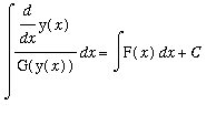 .
.
In general, the indefinite integral on the left-hand side will need to be evaluated with the Generalized Power Rule (with
 ). Finally, if an initial condition is supplied, it should be used now to obtain an equation for
 . If the antiderivatives work out particularly nice, it might be possible to solve for
 to obtain an explicit solution.
Enough of the general discussion. Let's look at a few specific examples.
Example 5: A First Separable Example
Find the general solution to the differential equation
| > |
alias( y=y(x) ):
ode5 := diff( y, x ) = -sqrt(x)/y:
ode5;
|

This differential equation cannot be solved by direct antidifferentiation, but is separable. Multiply the equation by
 yields

The indefinite integral, with respect to
 , of both sides of the separated equation leads to the equation
| > |
q2 := Int( lhs(q1), x ) = Int( rhs(q1), x ):
q2;
|

These integrals are fairly easy to evaluate by the Generalized Power Rule (with
 and
and
 ) and the Power Rule (with
 ). The result, after manually inserting a single constant of integration, is
| > |
q3 := value( lhs(q2) ) = value( rhs(q2) ) + C:
q3;
|

Other than multiplying this equation by 2

and replacing
 with a new constant, say
 ,
,
| > |
q5 := eval( q4, C=K/2 ):
q5;
|

there is about as simple as the general solution can be written. Taking the square root requires the consideration that
 could be positive or negative.
Example 6: Projectile Motion
An object moving in a straight line has acceleration (in centimeters per second per second) given by
| > |
A := a = 10*(1+t)^(-5) + 3*sin(Pi*t):
A;
|

Assume the object begins from rest with initial position
![s[0] = 10](images/DifferentialEqn68.gif) . Find the velocity and position of the object for any time
. Find the velocity and position of the object for any time
 > 0.
> 0.
Velocity
Acceleration is the rate of change (with respect to time) of velocity
| > |
alias( v=v(t) ):
ode6v := diff( v, t ) = rhs(A):
ode6v;
|

The general solution to this differential equation is obtained by direct integration
| > |
q1 := Int( lhs(ode6v), t ) = Int( rhs(ode6v), t ):
q1;
|

| > |
q2 := value( lhs(q1) ) = value( rhs(q1) ) + C:
q2;
|

The initial condition can be used to determine the particular solution with
 :
:
| > |
q3 := eval( q2, [ t=0, v=0 ] ):
q3;
|

| > |
q4 := isolate( q3, C ):
q4;
|

Thus, the velocity function is
| > |
V := eval( q2, q4 ):
V;
|

Position
The rate of change (with respect to time) of the position is the velocity:
| > |
alias( s=s(t) ):
ode6p := diff( s, t ) = rhs(V):
ode6p;
|

As with the acceleration this differential equation can be solved by direct integration:
| > |
q5 := Int( lhs(ode6p), t ) = Int( rhs(ode6p), t ):
q5;
|

| > |
q6 := value( lhs(q5) ) = value( rhs(q5) ) + K:
q6;
|

The initial condition can be used to determine the particular solution with
 :
:
| > |
q7 := eval( q6, [ t=0, s=10 ] ):
q7;
|

| > |
q8 := isolate( q7, K ):
q8;
|

Thus, the velocity function is
| > |
S := eval( q6, q8 ):
S;
|

Graphs of Solution
Graphs of the position, velocity, and acceleration over the 10 seconds of motion are shown below.
| > |
plot( [ rhs(A), rhs(V), rhs(S) ], t=0..10, color=[red,blue,green], legend=["acceleration","velocity","position"] );
|
![[Maple Plot]](images/DifferentialEqn84.gif)
Observe the oscillations in all three functions. For large t the acceleration and velocity become periodic. While the position oscillates, it is not periodic. Because the velocity oscillates about a positive constant (
 ) the position settles down to oscillations from a linear function.
Example 7: Wolf Population
The wolf population, W, in a certain state has been growing at a rate proportional to the cube root of the current population size. The population was estimated to be 1000 in 1980 and 1700 in 1990.
(a) Write the differential equation for the wolf population. Translate the two conditions into mathematical equations.
Let
 denote the time, in years, since 1980. The rate of change of the wolf population is diff( W(t), t ). Therefore, the differential equation governing this population is
| > |
alias( W=W(t) ):
ode7 := diff( W, t ) = k * W^(1/3):
ode7;
|

where
 is the constant of proportionality. The information about the population in 1980 and 1990 can be expressed as
| > |
eq1 := W(0) = 1000:
eq1;
|

| > |
eq2 := W(10) = 1700:
eq2;
|

(b) Solve the differential equation. Use the two conditions to determine values for the constant of proportionality and the integration constant.
This differential equation is separable:
| > |
q1 := ode7/W^(1/3):
q1;
|

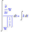
Now, the indefinite integral of each side with respect to
 is
is
| > |
q2 := Int( lhs(q1), t ) = Int( rhs(q1), t ):
q2;
|
Similar to Example 4, these integrals are fairly easy to evaluate by the Generalized Power Rule (with
 and
and
 ) and the Constant Rule. The result, after manually inserting a single constant of integration, is
| > |
q3 := value( lhs(q2) ) = value( rhs(q2) ) + C:
q3;
|

While it is possible to obtain an explicit formula for the wolf population,
| > |
q4 := isolate( q3, W );
|

it is not clear that this form is any easier to use.
To determine values for k and C, use the two data points provided in the problem description in the implicit solution. The resulting system of two (linear) equations for k and C is
| > |
q5 := eval( q3, [t=0,W=1000]):
q6 := eval( q3, [t=10,W=1700]):
q5;
q6;
|


Note: Comparison with Explicit Solution
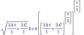
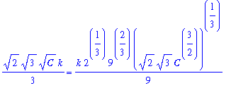
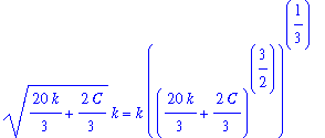
The system obtained from the implicit form of the solution to the differential equatin is much simpler than the system of equation that would be obtained if the explicit form of the solution were used:
| > |
eval( q4, [t=0,W=1000]);
eval( q4, [t=10,W=1700]);
|


The value of
 can be obtained from the first equation:
| > |
valC := isolate( simplify( q5 ), C ):
valC;
|

Inserting this value into the second equation, it is simple to solve for the proportionality constant:
| > |
valk := isolate( eval( q6, valC ), k ):
valk;
`` = evalf(rhs(valk));
|


The general solution can be validated as before:
| > |
q7 := eval( ode7, q4 ):
q7;
|

That the particular solution satisfies the two data points can be seen from
| > |
eval( q7, t=0 );
eval( q7, t=10 );
|


The wolf population is, therefore, modeled by the function
| > |
psol7 := eval( q4, [valC,evalf(valk)] ):
psol7;
|

(c) When, if ever, will the wolf population double from its population in 1990?
The equation that would be satisfied when the wolf population is 3400 is
| > |
q8 := eval( psol7, W=3400 );
|

The solution to this equation is
| > |
q9 := isolate( q8, t ):
q9;
`` = evalf(rhs(q9));
|


Thus, the wolf population will double in size in a little under 30 years, i.e., in 2009.
(d) According to this model, what is the long term prognosis for this wolf population?
The long-term behavior of this solution is governed by the exponent in this formula. Because this exponent is 3/2 > 1, and 4.224*t+100 > 0 for all t > 0, this model predicts the wolf population will grow without bound.
| > |
q10 := Limit( psol7, t=infinity ):
q10;
|


Example 8: Escape Velocity
The gravitational attraction
 exerted by Earth on an object with mass
 located at a distance
 from Earth's center is
| > |
alias( v=v, s=s ):
Fgrav := F = -m*g*R^2/s^2:
Fgrav;
|

where
 is Earth's radius and
 is the acceleration of gravaity at Earth's surface. Assume the initial velocity is
![v(0) = v[0]](images/DifferentialEqn121.gif) and neglect air resistance. For small values of
and neglect air resistance. For small values of
![v[0]](images/DifferentialEqn122.gif) an object launched from Earth's surface will return to Earth; for large values of
an object launched from Earth's surface will return to Earth; for large values of
![v[0]](images/DifferentialEqn123.gif) the object will not fall back to Earth. The escape velocity is the minimum value of
the object will not fall back to Earth. The escape velocity is the minimum value of
![v[0]](images/DifferentialEqn124.gif) for which the object does not return to Earth. Find the escape velocity as a function of
for which the object does not return to Earth. Find the escape velocity as a function of
 ,
,
 , and
, and
 .
.
Step 1: Modeling
Newton's Second Law of Motion states that

F = m*a
where F is the gravitational force between Earth and the launched object and a is the acceleration of the object. This gives
| > |
q1 := eval( N2, Fgrav );
|

Acceleration is the rate of change of velocity with respect to time and velocity is the rate of change of position with respect to time:
| > |
A := a = diff( v(t), t ):
A;
|

| > |
V := v(t) = diff( s(t), t ):
V;
|

This leads to the differential equation

Note that this differential equation is second order (i.e., it involves the second derivative of the unknown function. To reduce this equation to a first-order differential equation observe that
a = dv/dt = dv/ds ds/dt = dv/ds v.
The acceleration can therefore be expressed as
| > |
A2 := a = diff( v(s), s ) * v(s):
A2;
|

| > |
ode := eval( q1, A2 ):
ode;
|

This is better. The differential equation is first-order for v = v(s). Note that the independent variable is s and v=v(s) is the unknown function.
To complete the modeling step the initial data at time t=0 is
| > |
ic := [ s=R, v=v0 ]:
ic;
|
![[s = R, v = v0]](images/DifferentialEqn135.gif)
Step 2: Solution to Initial Value Problem
The differential equation in the initial value problem found in Step 1 is separable:
| > |
alias( v=v(s) ):
q3 := ode / m:
q3;
|

The indefinite integral of this equation with respect to s is
| > |
q4 := Int( lhs(q3), s ) = Int( rhs(q3), s ):
q4;
|

The antiderivatives are easily found using the
Antiderivative Rules -- and adding a constant.
| > |
gsol8 := value( lhs(q4) ) = value( rhs(q4) ) + C:
gsol8;
|

To determine the value of the constant that is consistent with the initial condition:
| > |
q5 := eval( gsol8, ic ):
q5;
|

Solve for the constant
| > |
q6 := isolate( q5, C ):
q6;
|

ans substitute this result into the general solution to obtain the particular solution in implicit form
| > |
q7 := eval( gsol8, q6 ):
q7;
|

| > |
psol8 := isolate( q7, v^2 ):
psol8;
|

Step 3: Analysis of Solution
If the object returns to Earth the velocity will be zero when the object reaches its maximum height. If the object does not return to Earth the velocity is never zero.
From the implicit form of the particular solution to the model for this problem it is seen that the velocity is zero when
| > |
q8 := eval( psol8, v=0 ):
q8;
|

This equation gives a formula for the maximum height of the object
| > |
smax := isolate( q8, s ):
smax;
|

Because s is the distance from the center of Earth,
 > 0. Therefore, this formula makes sense only when
| > |
q9 := denom( rhs(smax) ) > 0:
q9;
|

In terms of the initial velocity, which can be assumed to be positive, this requires
| > |
q10 := isolate( q9, v0 ) assuming v0>0:
q10;
|

If the initial velocity satisfies
![sqrt(2*g*R) <= v[0]](images/DifferentialEqn148.gif) then there is no maximum height. Thus, the escape velocity is
then there is no maximum height. Thus, the escape velocity is
![v[0] = sqrt(2*g*R)](images/DifferentialEqn149.gif) .
.
Lesson Summary
This lesson is an introduction to differential equations and their use as models to physical problems. The differential equations considered in this lesson could be solved by direct integration once the independent and dependent variables are separated. The general solution to a differential equation corresponds to a family of antiderivatives; a particular solution to an initial value problem is found by using additional information to identify a single function in the general solution that satisfies the differential equation and the initial condition. All solutions to differential equation can be checked by sustituting the proposed solution back into the differential equation.
What's Next?
To develop your differential equations skills, you are encouraged to take advantage of the practice sessions before you attempt the graded
online homework assignment. Work enough practice problems to master each concept, then complete the online homework assignment and the
assigned problems from the text. Independent practice sessions for a specific topic are also provided.
The next lesson,
Riemann Sums, is the first of two lessons devoted to the introduction of a second type of integral: the
Definite Integral. The final two sections of this Unit emphasize the intimate relationship between indefinite and definite integrals.

![]()
![]()
![]()
![]()
![]()
![]()
![]() is true for all values of
is true for all values of
![]() and so
and so
![]() is a solution to this differential equation.
is a solution to this differential equation.
![]()
![]() ,
,
![]() is
not
a solution to this differential equation.
is
not
a solution to this differential equation.
![]()
![]()
![]()
![]()
![]()
![]()
![]() and
and
![]() are also solutions to this differential equation while
are also solutions to this differential equation while
![]() is not a solution.
is not a solution.


 .
.
 .
.


![[Maple Plot]](images/DifferentialEqn84.gif)
 ) the position settles down to oscillations from a linear function.


 ) and the Constant Rule. The result, after manually inserting a single constant of integration, is


