The Definite Integral
The discussion of
Riemann sums in the previous lesson considers a number of different choices of partition of the interval [
![]() ,
,
![]() ] and of sample points (right, left, midpoint, random) within each subinterval. The examples suggest that, in the limit as the width of the partition decreases to zero, these choices are not important. That is, if the limit exists for one choice of partitions and sample points then it converges, with the same limit, for any choice of partition and sample points. When the function f is positive on the interval [
] and of sample points (right, left, midpoint, random) within each subinterval. The examples suggest that, in the limit as the width of the partition decreases to zero, these choices are not important. That is, if the limit exists for one choice of partitions and sample points then it converges, with the same limit, for any choice of partition and sample points. When the function f is positive on the interval [
![]() ,
,
![]() ], this limit is the area between the graph of
], this limit is the area between the graph of
![]() and the
and the
![]() -axis above the interval [
-axis above the interval [
![]() ,
,
![]() ]. More generally, these limits of Riemann sums are called
definite integrals
.
]. More generally, these limits of Riemann sums are called
definite integrals
.
| > |
-
f be a function defined on on a closed interval
![[a, b]](images/DefiniteInt9.gif) .
.
-
 be a partition of
![[a, b]](images/DefiniteInt11.gif) into
into
 subintervals with endpoints
-
the width of subinterval
 is
is
![Delta*x[i] = x[i]-x[i-1]](images/DefiniteInt21.gif)
-
the width of partition
 is
is
![Delta*x = max[i = 1 .. n]*Delta*x[i]](images/DefiniteInt23.gif)
-
![conjugate(x)[i]](images/DefiniteInt24.gif) is a point in subinterval
is a point in subinterval
 , i.e.,
![x[i-1]](images/DefiniteInt26.gif) <=
<=
![conjugate(x)[i]](images/DefiniteInt27.gif) <=
<=
![x[i]](images/DefiniteInt28.gif)
Definition ( Definite Integral )
Let
![]() =
=
![]() <
<
![]() <
<
![]() < ... <
< ... <
![]() <
<
![]() =
=
![]() .
.
The
definite integral
of a function f over an interval [
![]() ,
,
![]() ] is
] is
![Int(f(x),x = a .. b) = Limit(Sum(f(conjugate(x)[i])*Delta*x[i],i = 1 .. n),Delta*x = 0,right)](images/DefiniteInt31.gif)
provided the limit exists. When this definite integral exists it is said that f is
(Riemann) integrable on
[
![]() ,
,
![]() ].
].
| > |
| > |
At this point the only options for evaluating a definite integral are i) to use the definition in terms of limits and ii) to recognize the definite integral as the known area of a geometric region. One of the most important results in calculus is that definite integrals can be evaluated using an antiderivative of the integrand. The Fundamental Theorems of Calculus and Evaluating Definite Integrals lessons that conclude this unit contain this result and other techniques for the evaluation of definite integrals.
| > |
Example 1
In the Riemann Sums lesson the left, right, and two different random Riemann sums for
| > | f1 := x^2 - x + 2: f(x) = f1; |
![]()
on the interval [ 0, 3 ]
| > | a1 := 0: b1 := 3: |
all appeared to converge to the same value: 21/2. That is,
| > | Int( f1, x=a1..b1 ) = 21/2; |

| > | plot( f1, x=a1..b1 ); |
![[Maple Plot]](images/DefiniteInt36.gif)
| > |
Theorem 1
If f is a continuous function on the closed interval [
![]() ,
,
![]() ], then f is Riemann integrable on [
], then f is Riemann integrable on [
![]() ,
,
![]() ].
].
| > |
| > |
The class of integrable functions will be expanded later in this lesson. But, first, let's begin to develop some properties for definite integrals.
| > |
Property 1:

This does not require much discussion. So long as the integrand is finite at
![]() , the region will be a "rectangle" with height
, the region will be a "rectangle" with height
![]() and "width"
and "width"
![]() . The area of this rectangle is 0. Stated in terms of definite integrals:
. The area of this rectangle is 0. Stated in terms of definite integrals:
 .
.
| > |
Property 2:

Assume
![]() is a number between
is a number between
![]() and
and
![]() . Geometrically, this makes intuitive sense. If
. Geometrically, this makes intuitive sense. If
![]() >= 0 for all
>= 0 for all
![]() <=
<=
![]() <=
<=
![]() , then the area under the graph of
, then the area under the graph of
![]() over [
over [
![]() ,
,
![]() ] is the sum of the areas under the graph of
] is the sum of the areas under the graph of
![]() over [
over [
![]() ,
,
![]() ] and over [
] and over [
![]() ,
,
![]() ].
].
| > | P1 := plot( f1, x=0..2, color=cyan, filled=true ): P2 := plot( f1, x=2..3, color=pink, filled=true ): display( P1,P2, title="Int( f(x), x=0..3 ) = Int( f(x), x=0..2 ) + Int( f(x), x=2..3 )" ); |
![[Maple Plot]](images/DefiniteInt62.gif)
| > |
If the integrand has some negative values on [
![]() ,
,
![]() ], then it is not possible to use area to justify this property. Instead it is necessary to look at partitions.
], then it is not possible to use area to justify this property. Instead it is necessary to look at partitions.
| > |
Let
![]() be a partition of [
be a partition of [
![]() ,
,
![]() ] into n subintervals with endpoints
] into n subintervals with endpoints
![]() =
=
![]() <
<
![]() < ... <
< ... <
![]() <
<
![]() =
=
![]() with the property that
with the property that
![Limit(Sum(f(u[i])*Delta*u[i],i = 1 .. n),n = infinity) = Int(f(x),x = a .. b)](images/DefiniteInt74.gif)
and let
![]() be a partition of [
be a partition of [
![]() ,
,
![]() ] into n subintervals with endpoints
] into n subintervals with endpoints
![]() =
=
![]() <
<
![]() < ... <
< ... <
![]() <
<
![]() =
=
![]() with the property that
with the property that
![Limit(Sum(f(v[i])*Delta*v[i],i = 1 .. n),n = infinity) = Int(f(x),x = b .. c)](images/DefiniteInt84.gif) .
.
| > |
The points
![]() ,
,
![]() , ...
, ...
![]() ,
,
![]() ,
,
![]() , ... ,
, ... ,
![]() form a partition
form a partition
![]() of [ a, b ] into
of [ a, b ] into
![]() subintervals with widths
subintervals with widths
![]() and
and
![]() , for i = 1, 2, ..., n,. Then, for each integer
, for i = 1, 2, ..., n,. Then, for each integer
![]() ,
,
![Sum(f(x[i])*Delta*x[i],i = 1 .. 2*n) = Sum(f(x[i])*Delta*x[i],i = 1 .. n)+Sum(f(x[i])*Delta*x[i],i = n+1 .. 2*n)](images/DefiniteInt96.gif)
= .
![Sum(f(u[i])*Delta*u[i],i = 1 .. n)+Sum(f(v[i])*Delta*v[i],i = 1 .. n)](images/DefiniteInt97.gif)
and the linearity of limits yields
![Limit(Sum(f(x[i])*Delta*x[i],i = 1 .. 2*n),n = infinity) = Limit(Sum(f(x[i])*Delta*x[i],i = 1 .. n)+Sum(f(x[i])*Delta*x[i],i = n+1 .. 2*n),n = infinity)](images/DefiniteInt98.gif)
=
![Limit(Sum(f(u[i])*Delta*u[i],i = 1 .. n),n = infinity)+Limit(Sum(f(v[i])*Delta*v[i],i = n .. n),n = infinity)](images/DefiniteInt99.gif)
=

| > |
Now, because the original limit of Riemann sums over [
![]() ,
,
![]() ] exists, it can be identified and written as a definite integral. That is,
] exists, it can be identified and written as a definite integral. That is,
![Int(f(x),x = a .. b) = Limit(Sum(f(x[i])*Delta*x[i],i = 1 .. 2*n),n = infinity)](images/DefiniteInt103.gif)
=
 .
.
While this proof is valid only when
![]() <=
<=
![]() <=
<=
![]() , the result is true for any value of
, the result is true for any value of
![]() for which all three integrals exist.
for which all three integrals exist.
| > |
Example 2: Piecewise Continuous Integrand
Let a be a positive constant. Find the area of the regoin in the first quadrant bounded by the graph of
| > | f2 := piecewise( x>=0 and x<a, sqrt( 2*a*x-x^2 ), x>=a and x<= 3*a, (3*a-x)/2 ): f(x) = f2; |
![f(x) = PIECEWISE([(2*a*x-x^2)^(1/2), -x <= 0 and x-a < 0],[3/2*a-1/2*x, -x+a <= 0 and x-3*a <= 0])](images/DefiniteInt109.gif)
While it is not possible for Maple to graph this region in terms of the parameter
![]() , it can be graphed for specific values of
, it can be graphed for specific values of
![]() . For instance, with
. For instance, with
![]() , the region is:
, the region is:
| > | P3 := plot( eval(f2,a=2), x=0..6, scaling=constrained ): P3; |
![[Maple Plot]](images/DefiniteInt113.gif)
This region is clearly the union of a quarter circle and a triangle
| > | P4 := plot( eval(f2,a=2), x=0..2, color=pink, filled=true ): P5 := plot( eval(f2,a=2), x=2..6, color=cyan, filled=true ): display( P3,P4,P5 ); |
![[Maple Plot]](images/DefiniteInt114.gif)
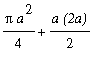
The area of the pink region is a quarter circle with radius 2. The area of the blue region is a triangle with base 4 and height 2. Therefore, by Property 2,
 =
=
![]() .
.
| > |
More generally, the region consists of the union of a quarter circle with radius
![]() above [ 0,
above [ 0,
![]() ] and a triangle with base
] and a triangle with base
![]() and height
and height
![]() above [
above [
![]() ,
,
![]() ]. Thus,
]. Thus,

=

=
=
 .
.
| > |
Theorem 2
If f is a piecewise continuous function on the interval [
![]() ,
,
![]() ], then f is (Riemann) integrable on [
], then f is (Riemann) integrable on [
![]() ,
,
![]() ].
].
Sketch of Proof
Divide the interval [
![]() ,
,
![]() ] into a finite number of nonoverlapping intervals,
] into a finite number of nonoverlapping intervals,
![]() ,
,
![]() , ...,
, ...,
![]() , on which f is continuous. Then, by Theorem 1, f is integrable on each of the smaller intervals. Property 2 tells us the sum of these definite integrals is the definite integral over [
, on which f is continuous. Then, by Theorem 1, f is integrable on each of the smaller intervals. Property 2 tells us the sum of these definite integrals is the definite integral over [
![]() ,
,
![]() ]. Since this definite integral exists, f must be (Riemann) integrable on the full interval, [
]. Since this definite integral exists, f must be (Riemann) integrable on the full interval, [
![]() ,
,
![]() ].
].
| > |
| > |
Example 3: A Nonintegrable Function
Consider the function
![f(x) = PIECEWISE([1, x*` rational`],[0, x*` irrational`])](images/DefiniteInt140.gif)
| > |
Recall that between any two rational numbers there is at least one irrational number and that between any two irrational numbers there is at least one rational number. Due to the way rational and irrational numbers are interspersed, it is not possible to create an instructive plot of this function. In fact, because every floating-point number representable in a computer is rational, a computer-generated plot would look like the horizontal line
![]() .
.
| > |
Let
![]() be the partition of [ 0, 1 ] into n subintervals with
be the partition of [ 0, 1 ] into n subintervals with
![x[i] = i/n](images/DefiniteInt143.gif) . Then
. Then
![]() =
=
![]() for all
for all
![]() . Because every subinterval contains a rational number the largest value of f on the subinterval is 1. Thus, the upper Riemann sum on
. Because every subinterval contains a rational number the largest value of f on the subinterval is 1. Thus, the upper Riemann sum on
![]() is
is
![U[n] = Sum(1*Delta*x[i],i = 1 .. n)](images/DefiniteInt148.gif) =
=
 .
.
Likewise, the smallest value on every subinterval is 0 and the lower Riemann sum of
![]() is
is
![L[n] = Sum(0*Delta*x[i],i = 1 .. n)](images/DefiniteInt151.gif) =
=
 .
.
While the sequence of upper Riemann sums converges to 1 and the sequence of lower Riemann sums converges to 0, the fact that the upper and lower Riemann sums for the same function and interval do not converge to the same value means that this function is not Riemann integrable.
| > |
| > |
The function in Example 3 is unlike any other function encountered in this course. It is included here only to show that there are, in fact, some functions that are not integrable. You will not encounter another function like this in this course -- well, there might be something like this in the online homework.
| > |
Property 3:

By Property 2 it is known that
 .
.
By Property 1 the left-hand side of this equation is 0. Thus,

and so
 .
.
| > |
Property 4:

Linearity of the definite integral is a direct consequence of the linearity of limits and sums:
![Int(r*f(x)+s*g(x),x = a .. b) = Limit(Sum(r*f(x[i])+s*g(x[i]),i = 1 .. n),n = infinity)](images/DefiniteInt158.gif)
=
![Limit(r*Sum(f(x[i]),i = 1 .. n)+s*Sum(g(x[i]),i = 1 .. n),n = infinity)](images/DefiniteInt159.gif)
=
![r*Limit(Sum(f(x[i]),i = 1 .. n),n = infinity)+s*Limit(Sum(g(x[i]),i = 1 .. n),n = infinity)](images/DefiniteInt160.gif)
=
 .
.
| > |
Example 4
In Example1 it was determined that
 .
.
Use the properties of definite integrals to determine
 .
.
| > |
Linearity of the definite integral, Property 4, allows us to write

=

The definite integral on the left is known (from Example 1). The second and third integrals on the right hand side can be determined by geometry:

| > | plot( x, x=0..3, color= pink, filled=true ); |
![[Maple Plot]](images/DefiniteInt167.gif)
The area of the right triangle with base3 and height 3 is
 =
=
![]() (3) (3) =
(3) (3) =
![]() .
.
| > |

| > | plot( 1, x=0..3, color=cyan, filled=true, view=[DEFAULT,0..3] ); |
![[Maple Plot]](images/DefiniteInt172.gif)
The area of the rectangle with base 3 and height 1 is
 = 3 ( 1 ) = 3.
| > |
Therefore,

=

= 9.
| > |
| > |
![Int(f(x),x = a .. b) = Limit(Sum(f(conjugate(x)[i])*Delta*x[i],i = 1 .. n),Delta*x = 0,right)](images/DefiniteInt176.gif)


