Lesson Overview
The processes for evaluating limits described in the
Conceptual Understanding of the Limit lesson can be summarized in the following informal definition:
Definition: Informal Definition of Limit
The statement
 means the difference between
 and
and
 can be made as small as desired for all values of
 sufficiently close to -- but different from --
 .
.
The development of general tools for working with and applying limits requires a more precise definition of limit. The following definition provides a framework upon which we will be able to develop a wide range of useful techniques.
Definition: Precise, or
 , Definition of Limit
 if and only if for every
 > 0 there exists a number
 > 0 with the property that
if 0 <
 <
<
 (and
(and
 is in the domain of f), then
 <
<
 .
.
This definition can be difficult to understand. Do not be concerned if it does not make sense to you right now. The structure of this lesson has designed to help you understand the definition and be able to apply it in some cases.
The first step is to develop a graphical interpretation of the precise definition. Next, the algebraic manipulations involved in applying the precise definition will be explored for four examples. The lesson concludes with a brief discussion of one-sided limits.
Graphical Interpretation of the Limit
The precise definition of a limit looks pretty imposing. The definition becomes much more understandable when it can be expressed graphically. The
EpsilonDelta
maplet [
Maplet Viewer] [
MapleNet] provides an excellent interface for visualizing the roles of
 and
and
 and for obtaining, as a result, a theoretical understanding of limits.
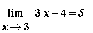
Example 1:
1. Follow these steps:
-
Start the
EpsilonDelta
maplet [
Maplet Viewer] [
MapleNet]
-
In the top row of the interface, enter the function as:
3*x-4
, a =
3
, and
L
=
5
.
-
Set the plot ranges to
xmin
=
0
,
xmax
=
5
,
ymin
=
0
, and
ymax
=
10
.
-
Set
epsilon
=
0.50
and
delta
=
0.50
(either enter these values in the boxes or use the slider to come close to these values)
-
Click on the
Plot
button at the bottom of the Maplet window.
Note that the blue horizontal strip is not contained within the red lines. This means this value of is too large to satisfy the conditions in the definition of the limit.
2. Change the value of
delta
to
0.05
.
Now the blue horizontal strip falls entirely within the red lines. This value of does satisfy the conditions in the definition of the limit.
But, this is not enough! The definition states that it must be possible to find such a for every
 > 0. At present we have shown this property is true only for
 = 0.5.
3. Find (exactly or approximately) the largest value of
 for which the conditions of the definition of the limit are satisfied for
 = 0.50.
4. Repeat 3. for
 = 0.25. (You might to try
 = 0.1 and
 =0.05 to get started.)
5. Can you make any conjectures about a general rule for selecting
 for any given
 ?
?
Example 2:

1. Consider the same limit, but with an incorrect value for the limit (say,
L
=
2
).
2. Choose a (positive) value for
 .
.
3. Can you find a value of
 that satisfies the conditions of the definition of a limit?
If you can find one value of
 > 0 for which the conditions are not satisfied, this proves that this value of is incorrect. The limit either has a different value or does not exist.
Example 3:
1. Find the value of this limit.
2. Find values of
 that satisfy the conditions of the definition for
 = 0.50,
 = 0.25, and
 = 0.10.
3. Attempt to find a general formula for
 in terms of
 that satisfies the conditions of the definition.
Example 4:
1. Choose a value for
 with
with
 > 1. Explain why all
 > 0 satisfy the conditions in the definition.
2. Set
 = 0.50. How small must
 be to satisfy the conditions in the definition?
3. Repeat 2. with
 = 0.25 and
 = 0.10.
4. Can you find a general formula for
 that works for all
 > 0?
> 0?
Example 5:
1. Find the value of this limit (if it exists).
2. Find values of
 that satisfy the conditions of the definition for
 = 0.50,
 = 0.25, and
 = 0.10.
Having completed these five examples, you are now ready to learn how to use the definition of limits to prove that a limit has a given value.
Writing
 Proofs for Limits
The graphical interpretation of the definition should have provided a better understanding of the roles of
 and
and
 in the precise definition of a limit.
Equipped with this understanding it is now appropriate to look at a few ``
 proofs'' of limits. Examples 6-9 present
 proofs for increasingly complicated functions. As you work through these examples, be sure to test your formulae for
 in the
EpsilonDelta
maplet [
Maplet Viewer] [
MapleNet].
in the
EpsilonDelta
maplet [
Maplet Viewer] [
MapleNet].
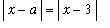
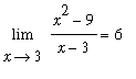
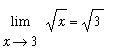
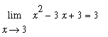
Example 6: Linear Function
Consider the statement that
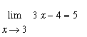 . (This limit has been seen previously in Example 1 of this lesson.) To prove that this statement is correct introduce


Our goal is to show that, for any
 > 0, is it possible to find a positive value of delta that assures that if it is given that
| > |
given := abs( x-a ) < delta:
given;
|

then
| > |
goal := abs( f-L ) < epsilon:
goal;
|

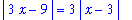
The typical proof begins by looking at the left-hand side of the goal:
| > |
start := lhs( goal ):
start;
|

and attempting to identify ways in which this can be bounded by a constant times a power of
 . The most common way of introducing
 into this expression is to locate factors of .
 . In this example, it is easy to see that:
| > |
q1 := start = 3*abs(x-3):
q1;
|
and so
| > |
q2 := rhs(q1) < 3*delta:
q2;
|
At this point we have shown that
| > |
q3 := start < rhs(q2):
q3;
|
If it is possible to choose
 so that
| > |
constraint := rhs(q3) < epsilon:
constraint;
|

then the proof will be complete. In this case, the above constraint is satisfied whenever
| > |
isolate( constraint, delta );
|

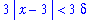
This process shows that, given any
 >0:
>0:
if 0 <
 <
<
 then
then
 <
<
 < 3 (
< 3 (
 ) =
) =
 .
.
This concludes the proof of this limit.
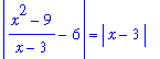
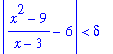
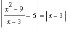
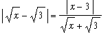
Example 7: Rational Function at a Removable Singularity
Consider the statement that
 . To prove that this statement is correct introduce


Our goal is to show that, for any
 > 0, is it possible to find a positive value of delta that assures that if it is given that
| > |
given := abs( x-a ) < delta:
given;
|

then
| > |
goal := abs( f-L ) < epsilon:
goal;
|
The proof begins as in Example 1 by looking at the left-hand side of the goal:
| > |
start := lhs( goal ):
start;
|

and attempting to identify ways in which this can be bounded as in Example 1. The most common way of introducing
 into this expression is to locate factors of
 . This takes a little more effort than in the previous example. First, note that the condition 0 <
 <
<
 implies that
 and so there is no problem with division by zero. With this potential problem alleviated, find a common denominator and simplify:
| > |
q1 := start = simplify( start ) assuming x<>3:
q1;
|
and so
| > |
q2 := rhs(q1) < delta:
q2;
|

At this point we have shown that
| > |
q3 := start < rhs(q2):
q3;
|
If it is possible to choose
 so that
| > |
constraint := rhs(q3) < epsilon:
constraint;
|

then the proof will be complete. In this case, the above constraint is satisfied whenever
| > |
isolate( constraint, delta );
|

This process shows that, given any
 >0:
>0:
if 0 <
 <
<
 then
then
 <
<
 <
<
 .
.
This concludes the proof of this limit.
Example 8: Power Function
Consider the statement that
 . To prove that this statement is correct introduce


Our goal is to show that, for any
 > 0, is it possible to find a positive value of delta that assures that if it is given that
| > |
given := abs( x-a ) < delta:
given;
|

then
| > |
goal := abs( f-L ) < epsilon:
goal;
|

The proof begins as in Examples 1 and 2 by looking at the left-hand side of the goal:
| > |
start := lhs( goal ):
start;
|

and attempting to identify ways in which this can be bounded as in the previous examples. The most common way of introducing
 into this expression is to locate factors of
 . This takes a little more effort than in the previous examples. But first, one technicality needs to be addressed. The quantity
 is defined (as a real number) only when
 >= 0. This is where the parenthetic remark about
 being in the domain of the function is needed. In this case the condition 0 <
 <
<
 must be amended with
 >= 0 to ensure that the expression
 makes sense.
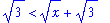
Observe that
 =
=
 =
=
 and so
 . When absolute values are applied:
| > |
q1 := start = abs((x-3))/abs(sqrt(x)+sqrt(3)):
q1;
|

Our focus is now directed towards the denominator on the right-hand side of the previous expression.
| > |
d1 := denom( rhs(q1) ):
d1;
|

First,
 is always positive so the absolute values are not needed:
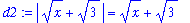
Moreover, because
 > 0, we see that
| > |
d3 := rhs(d2) > sqrt(3):
d3;
|
Taking reciprocals (and noting that Maple has converted the inequality to a <):
| > |
bound := 1/lhs(d3) > 1/rhs(d3):
bound;
|
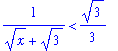
We are now ready to return the full quotient. Recall that

The numerator on the right-hand side can be bounded above by epsilon, the remaining term is bounded by the previous argument. The result is
| > |
q2 := rhs(q1) < delta*rhs(bound):
q2;
|
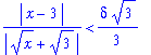
At this point we have shown that
| > |
q3 := start < rhs(q2):
q3;
|
If it is possible to choose
 so that
| > |
constraint := rhs(q3) < epsilon:
constraint;
|

then the proof will be complete. In this case, the above constraint is satisfied whenever
| > |
isolate( constraint, delta );
|

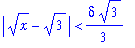
This process shows that, given any
 >0:
>0:
if 0 <
 <
<
 (and
(and
 >= 0) then
 <
<
 <
<
 .
.
This concludes the proof of this limit.
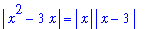
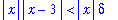
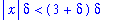
Example 9: Quadratic Function
Consider the statement that
 . (This limit has been seen previously in Example 3 of this lesson.) To prove that this statement is correct introduce


Our goal is to show that, for any
 > 0, is it possible to find a positive value of delta that assures that if it is given that
| > |
given := abs( x-a ) < delta:
given;
|

then
| > |
goal := abs( f-L ) < epsilon:
goal;
|

The proof begins as in all previous examples by looking at the left-hand side of the goal:
| > |
start := lhs( goal ):
start;
|

The appearance of
 in this expression is fairly obvious:
| > |
q1 := start = abs(x)*abs(x-3):
q1;
|
Applying the assumption that
 <
<
 leads to:
| > |
q2 := rhs(q1) < abs(x)*delta:
q2;
|
It now remains to deal with the term
 on the right-hand side of this equation. The general approach is similar to that takin in Example 3 but the details are a little more involved. The key is to observe that the condition 0 <
 <
<
 can be written equivalently as
 <
<
 <
<
 (and
(and
 ) or
) or
 <
<
 <
<
 . Now, because
 ,
,
 >
>
 and so
 <
<
 .
.
| > |
q3 := rhs(q2) < (3+delta)*delta:
q3;
|
If it is possible to choose
 so that
| > |
constraint := rhs(q3) < epsilon:
constraint;
|

then the proof will be complete. In this case, the above constraint is satisfied whenever
| > |
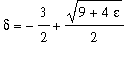
solve( constraint, delta );
|
Well, the fact that Maple's response is empty means that Maple was unable to solve this inequality. If the inequality is converted to an equality
| > |
c2 := convert( constraint, equality ):
c2;
|

it becomes apparent that this is a quadratic in
 (with
(with
 as a parameter). The two roots are
| > |
r := solve( c2, delta );
|
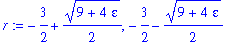
These roots are real because
 >0. Moreover, one is positive and one is negative. It is not too difficult to now determine that the constraint is satisfied for all
 with 0 <
 <
<
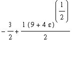 .
.
This process shows that, given any
 >0:
>0:
if 0 <
 <
<
 then
then
 <
<
 <
<
 .
.
This concludes the proof of this limit.
![MATRIX([[`Type of Limit`, `Values of Independent Variable (Compact Form)`, `Values of Independent Variable (Long Form)`], [_____________, _________________________________________, ____________________...](images/LimitPrecise194.gif)
 should contain the following features:
![[Maple Plot]](images/LimitPrecise206.gif)