Next: Visualizaton Tools and the Up: Tutorial #3: A Remote Previous: Setting up the Local
![]()
![]()
![]()
![]()
Next: Visualizaton
Tools and the Up: Tutorial
#3: A Remote Previous: Setting
up the Local
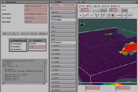
Select the Remote ![]() Connection widget and enter the (1) internet address of the remote
server (i.e. Host), (2) 'cd Celia_server; pexec us3d -sz 4' in the Application
text field, (3) user name and (4) password. Selecting Start initiates
the remote commands on the server. (See Figure 16)
In the text window, the direct output is displayed. Once registration of
variables (Tracking) and Parameters (Steering) is complete,
select the Connection button to register the corresponding variables
on your client workstation.
Connection widget and enter the (1) internet address of the remote
server (i.e. Host), (2) 'cd Celia_server; pexec us3d -sz 4' in the Application
text field, (3) user name and (4) password. Selecting Start initiates
the remote commands on the server. (See Figure 16)
In the text window, the direct output is displayed. Once registration of
variables (Tracking) and Parameters (Steering) is complete,
select the Connection button to register the corresponding variables
on your client workstation.
Figure 16: Connection Interface Widget
Select the Remote ![]() Variables widget which lists all registered tracking variables.
You may enter any time step in the Time Index text field for variables
that have been computed. An option for 3D data compression may be selected
for transfer of large data sets. The value of -1 selects
data for the current time step. You may select either variables `pressure'
or `concentration', remembering that the Min-Max values of the
color map need to be adjusted accordingly. Additional data from individual
processors are also available for debugging and observing solver behavior.
Variables widget which lists all registered tracking variables.
You may enter any time step in the Time Index text field for variables
that have been computed. An option for 3D data compression may be selected
for transfer of large data sets. The value of -1 selects
data for the current time step. You may select either variables `pressure'
or `concentration', remembering that the Min-Max values of the
color map need to be adjusted accordingly. Additional data from individual
processors are also available for debugging and observing solver behavior.
First set the color map text fields in the Main Window to Min=-30
and Max=70 and select the current pressure data by entering -1 into
the Remote ![]() Variables widgets Time Index text field and selecting pressure.
In the Main Window, advance the time control to view the current pressure
field.
Variables widgets Time Index text field and selecting pressure.
In the Main Window, advance the time control to view the current pressure
field.
Next change the color map text field to Min=0. and Max=.01.
Select the current concentration data by entering -1 into the Remote
![]() Variables widgets Time Index text field and selecting concentration.
Previous time-indexed concentration data sets may be retrieved and viewed
at any time. Requesting them will automatically load them into G3D
and overwrite previous data with that time index. You may use the Delete
button in the Main Window to delete unwanted data with the current Time
Index.
Variables widgets Time Index text field and selecting concentration.
Previous time-indexed concentration data sets may be retrieved and viewed
at any time. Requesting them will automatically load them into G3D
and overwrite previous data with that time index. You may use the Delete
button in the Main Window to delete unwanted data with the current Time
Index.
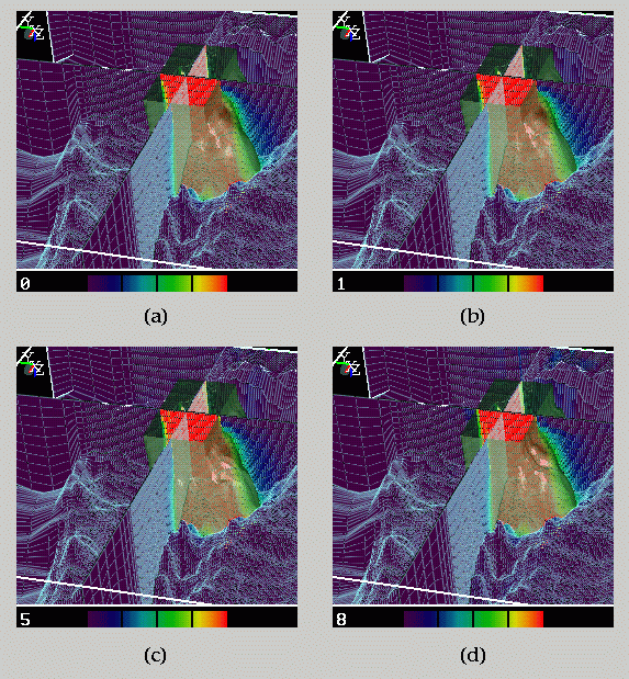
The results of using a 3D data compression option (using Remote
![]() Compression) are illustrated in Figure 17
for a refined version (129x137x11) of the Celia data set
which was used in Tutorial 1. Figure 17.a
shows the results of rendering the original data set while Figure 17.d
is a rendering of the data file reconstructed after lossy compression by
a factor of 1200. 3D
Data Compression is not included in all distributions. Please contact
Bob Sharpley (sharpley@math.sc.edu) for more information.
Compression) are illustrated in Figure 17
for a refined version (129x137x11) of the Celia data set
which was used in Tutorial 1. Figure 17.a
shows the results of rendering the original data set while Figure 17.d
is a rendering of the data file reconstructed after lossy compression by
a factor of 1200. 3D
Data Compression is not included in all distributions. Please contact
Bob Sharpley (sharpley@math.sc.edu) for more information.
To illustrate the capability of steering, select the Start button
of the Connection widget. After variables and parameters are registered
(observe the direct output text window in the widget), select Connect.
Select Remote ![]() Parameters to bring up the widget of all registered parameters.
In this tutorial, only the concentration level of a specific cell is registered.
Change its value to 1 and enter Return. Select an additional slice of y=2
in the Tools
Parameters to bring up the widget of all registered parameters.
In this tutorial, only the concentration level of a specific cell is registered.
Change its value to 1 and enter Return. Select an additional slice of y=2
in the Tools ![]() Slice widget to observe the effect of introducing an additional
contaminant at that location.
Slice widget to observe the effect of introducing an additional
contaminant at that location.
|
Figure 17: |
Comparison of Compressed Data to original Scalar Field: a) Original data and Compression Rates of b) 172, c) 493, and d) 1200 times compression. |
See the Frequently Asked Questions file (`FAQ'),
which is included in the Interactive
Controller library distribution, if there are problems with communication
or security issues at a particular site. Several workarounds for facilties
with firewalls are described.
![]()
![]()
![]()
![]()
Next: Visualizaton
Tools and the Up: Tutorial
#3: A Remote Previous: Setting
up the Local