lab12.mws --- Sequences of Functions: Convergence
| > |
restart;
with( plots ):
|
Warning, the name changecoords has been redefined
Auxiliary Procedures (execute, but do not change)
| > |
DisplayPtSeq := proc( F, Terms )
local Domain, L, P1, P2, n, terms, pts;
n := lhs(Terms);
terms := rhs(Terms);
Domain := min(op(terms))..max(op(terms));
pts := [seq( [k,eval(F,[n=k])], k=terms )];
P1 := plot( pts, style=point, symbol=circle, color=blue );
if nargs>2 then
L := args[3];
P2 := plot( L, Domain, color=cyan, thickness=2 );
else
L := NULL;
P2 := NULL;
end if:
return plots[display]( [P1, P2], view=[Domain,DEFAULT] )
end proc:
|
| > |
AnimateFnSeq := proc( F, Terms, Domain )
local n, terms, f, G, P;
n := lhs(Terms);
terms := rhs(Terms);
f := unapply( F, n );
if nargs>3 then G := args[4] else G := NULL end if:
P := [seq( plot( [f(n),G], Domain, title=sprintf("n=%a",n) ), n=terms )];
plots[display]( P, insequence=true )
end proc:
|
| > |
DisplayFnSeq := proc( F, Terms, Domain )
local n, terms, f, G, P;
n := lhs(Terms);
terms := rhs(Terms);
f := unapply( F, n );
if nargs>3 then G := args[4] else G := NULL end if:
P := plot( [seq(f(n),n=terms),G], Domain );
plots[display]( [P] )
end proc:
|
Lab Overview
Limits have been the foundation for almost everything you have studied thus far in calculus. To date, all of these limits have been of one of two types: the limit of a function as the independent variable approaches a specific value --
 -- or the limit of a sequence of numbers --
![limit(a[n],n = infinity) = A](images/lab122.gif) .
.
This lab introduces a new type of limit -- the limit of a sequence of functions:
,n = infinity) = g(x)](images/lab123.gif) .
.
Note, in particular, that the value of this limit will be a
function
. That is, the limit might depend on
 (but cannot depend on
 ).
).
Another distinguishing feature of sequences of functions is that there are different types of convergence.
Definition: Convergence in Norm
Let
![{f[n], n = 1 .. infinity}](images/lab126.gif) be a sequence of functions defined on an interval
be a sequence of functions defined on an interval
![[a, b]](images/lab127.gif) . We say the sequence
. We say the sequence
![{f[n]}](images/lab128.gif) converges in norm on
converges in norm on
![[a, b]](images/lab129.gif) to a function g if
to a function g if
-g(x))^2,x = a .. b),n = infinity) = 0](images/lab1210.gif) .
.
Notes:
1. For every integer
 , define
![V[n] = Int(abs(f[n](x)-g(x))^2,x = a .. b)](images/lab1212.gif) . Observe that
. Observe that
![V[n]](images/lab1213.gif) is a number (provided the integral exists).
is a number (provided the integral exists).
2. The limit that appears in this definition is the limit of a sequence of numbers:
![limit(V[n],n = infinity)](images/lab1214.gif) .
.
If this limit is not zero or does not exist, then the sequence of functions does not converge in norm on
![[a, b]](images/lab1215.gif) to g.
to g.
Definition: Pointwise Convergence
Let
![{f[n], n = 1 .. infinity}](images/lab1216.gif) be a sequence of function defined on an interval
be a sequence of function defined on an interval
![[a, b]](images/lab1217.gif) . The sequence
. The sequence
![{f[n]}](images/lab1218.gif) is said to
converge pointwise on
is said to
converge pointwise on
![[a, b]](images/lab1219.gif) to
g if, for
every
to
g if, for
every
 in
in
![[a, b]](images/lab1221.gif) ,
,
-g(x),n = infinity) = 0](images/lab1222.gif) .
.
Notes:
1. Pointwise converge requires consideration of the sequence of numbers
, n = 1 .. infinity}](images/lab1223.gif) where
where
 is a number in
![[a, b]](images/lab1225.gif) .
.
2. Because there are an infinite number of points in
![[a, b]](images/lab1226.gif) this calls for the consideration of an infinite number of sequences.
this calls for the consideration of an infinite number of sequences.
3. In light of Note 2 above, it is impossible to check for pointwise convergence by direct calculation.
Uniform Convergence
Let
![{f[n], n = 1 .. infinity}](images/lab1227.gif) be a sequence of functions defined on an interval
be a sequence of functions defined on an interval
![[a, b]](images/lab1228.gif) . The sequence
. The sequence
![{f[n]}](images/lab1229.gif) is said to
converge uniformly on
is said to
converge uniformly on
![[a, b]](images/lab1230.gif) to
g if
to
g if
![limit(max[` x = [a, b] `]*abs(f[n](x)-g(x)),n = infinity) = 0](images/lab1231.gif)
Notes:
1. For each integer
 , define
![B[n]](images/lab1233.gif) to be the maximum value of
to be the maximum value of
-g(x))](images/lab1234.gif) on the interval
on the interval
![[a, b]](images/lab1235.gif) . That is,
. That is,
![B[n] = max[` x=[a,b] `]*abs(f[n](x)-g(x))](images/lab1236.gif) .
.
2. The sequence
![{f[n]}](images/lab1237.gif) converges uniformly to g if and only if
converges uniformly to g if and only if
![limit(B[n],n = infinity)](images/lab1238.gif) .
.
The examples provide graphical and other intuitive interpretations of the different types of convergence. It is particularly important to understand the connections between the different types of convergence. The Lab Questions will ask you to answer some questions about these examples.
Continuing the practice started last week, this lab assignment includes a separate and explicit integration problem. You are encouraged to use the
Integration
maplet [
Maplet Viewer][
MapleNet] to help with this problem.
Deadline for submitting a lab solution is midnight, Thursday, April 10, 2003.
Example 1:
Consider the sequence of functions
| > |
F1 := (1-x^2)^(1/2+1/(2*n)):
f[n](x) = F1;
|
 = (1-x^2)^(1/2+1/(2*n))](images/lab1239.gif)
on the interval [ -1, 1 ].
Initial Investigation
The following command creates a nice picture of the first few terms of the sequence of functions
| > |
DisplayFnSeq( F1, n=[1,2,4,8,16], x=-1..1 );
|
![[Maple Plot]](images/lab1240.gif)
This picture suggests that the functions do approach some limit. To determine this limit, note that the only place
 appears in the functions is the exponent and the exponents converge to
 as
as
 approaches
 . This suggests that the limit function should be
| > |
G1 := sqrt(1-x^2):
g(x) = G1;
|
Confirmation that this is the correct limit can be obtained from the following animation
| > |
AnimateFnSeq( F1, n=[1,2,4,8,16], x=-1..1, G1 );
|
![[Maple Plot]](images/lab1246.gif)
The visual "convergence" shown in these plots needs to be translated into the language introduced at the beginning of this lab. Is the convergence uniform, pointwise, or in the norm?
Pointwise Convergence
Recall that pointwise convergence occurs when, for every possible
 in [-1,1], the sequence of function values at
 converges. As pointed out previously, it is not possible to do this check for
every
possible value of
converges. As pointed out previously, it is not possible to do this check for
every
possible value of
 in [-1,1]. But, to check the convergence at selected values of
 , say
, say
 , use a plot of the sequence of numbers
, n = 1 .. infinity}](images/lab1252.gif) :
:
| > |
DisplayPtSeq( eval(F1, x=1/2), n=[1,2,4,8,16,32,64,128], eval(G1,x=1/2) );
|
![[Maple Plot]](images/lab1253.gif)
Change the
 in the above command to other points in [-1,1]. Can you find any values of
 that do not converge to
 ? These results provide a strong indication that
, n = 1 .. infinity}](images/lab1257.gif) converges pointwise to
converges pointwise to
 .
.
An alternate approach to pointwise convergence is to examine the sequence
-g(x)), n = 1 .. infinity}](images/lab1259.gif) .
.
| > |
DisplayFnSeq( abs(F1-G1),n=[1,2,4,8,16,32,64, 128, 256, 512,1024],x=-1..1 );
|
![[Maple Plot]](images/lab1260.gif)
Pointwise convergence on [-1,1] is seen in the fact that the difference approaches zero for every point in the interval.
Uniform Convergence
The last plot in the discussion of pointwise convergence suggests that for each
 ,
,
-g(x))](images/lab1262.gif) has a maximum value at two (symmetric) points. The location of the maximum values depends on
has a maximum value at two (symmetric) points. The location of the maximum values depends on
 . But, the value of the maximum error on [-1,1] approaches zero as
 ->
->
 . This is uniform convergence!
The same conclusion can be reached using the animation of
-g(x))](images/lab1266.gif) :
:
| > |
AnimateFnSeq( abs(F1-G1),n=[1,2,4,8,16,32,64, 128, 256, 512,1024],x=-1..1 );
|
![[Maple Plot]](images/lab1267.gif)
Convergence in the Norm
To investigate convergence in norm it is necessary to look at the sequence of numbers,
![V[n]](images/lab1268.gif) , defined by
, defined by
| > |
V1 := Int( (F1-G1)^2, x=-1..1 ):
V[n] = V1;
|
![V[n] = Int(((1-x^2)^(1/2+1/(2*n))-(1-x^2)^(1/2))^2,x = -1 .. 1)](images/lab1269.gif)
These integrals are not easy to evaluate, but Maple can help us to visualize the terms in this sequence:
| > |
DisplayPtSeq( V1, n=[1,2,4,8,16,32,64,128,256,512,1024] );
|
![[Maple Plot]](images/lab1270.gif)
These terms clearly decay to zero as n increases. That is,
-g(x))^2,n = infinity) = 0](images/lab1271.gif) . This means this sequence converges in the norm to
. This means this sequence converges in the norm to
 on [-1,1].
Example 2:
Consider the sequence of functions
| > |
F2 := piecewise(x<n,1/(1+(x-n)^2),x>=n,1):
f[n](x) = F2;
|
 = PIECEWISE([1/(1+(x-n)^2), x < n],[1, n <= x])](images/lab1273.gif)
on the entire real line.
Initial Investigation
The first few terms of the sequence of functions
| > |
DisplayFnSeq( F2, n=[$1..16], x=-1..20 );
|
![[Maple Plot]](images/lab1274.gif)
It is difficult to determine the limit directly from the definition of the functions in this sequence. However, after a little thought it should become apparent that the limit at every point the plots of the first few functions suggest that the (pointwise) limit at every point is zero. That is,

Pointwise Convergence
The argument leading to the limiting function is really an argument that the sequence converges pointwise to the zero function. Additional evidence in support of this conclusion can be obtained by looking at the sequence of function values for a specific value of
 , say
, say
 :
:
| > |
DisplayPtSeq( eval(F2,x=20), n=[1,2,4,8,16, 32,64,128], 0 );
|
![[Maple Plot]](images/lab1278.gif)
Look at similar plots for other values of
 . Assuming
 , the first few terms are 1 but eventually (
 >
>
 ) the sequences exhibit very rapid decay to zero. This is pointwise convergence. The following animation provides another view of this sequence of functions.
| > |
AnimateFnSeq( F2, n=[1,2,4,8,16,32,64,128,256], x=-1..300 );
|
![[Maple Plot]](images/lab1283.gif)
Based on these two views of the sequence, it is clear that the pointwise limit of the sequence of functions is
 .
.
Uniform Convergence
Turning our attention to uniform convergence,
-g(x)) = 1](images/lab1285.gif) for all
for all
 >=
>=
 . Thus, the maximum difference between a function in the sequence and the zero function (the proposed limit) is always 1. In particular,
-g(x)),n = infinity) = limit(1,n = infinity)](images/lab1288.gif) =
=
 .
.
This means
![f[n]](images/lab1290.gif) does not converge uniformly to
does not converge uniformly to
 .
.
Convergence in the Norm
To investigate convergence in norm it is necessary to look at the sequence of numbers,
![V[n]](images/lab1292.gif) , defined by
, defined by
| > |
V2 := Int( (F2-0)^2, x=-infinity..infinity ):
V[n] = V2;
|
![V[n] = Int(PIECEWISE([1/(1+(x-n)^2), x < n],[1, n <= x])^2,x = -infinity .. infinity)](images/lab1293.gif)
Observe that these integrals can be broken into two pieces
| > |
V2a := Int( 1/(1+(x-n)^2)^2, x=-infinity..n ):
V2b := Int( 1^2, x=n..infinity ):
V[n] = V2a + V2b;
|
![V[n] = Int(1/((1+(x-n)^2)^2),x = -infinity .. n)+Int(1,x = n .. infinity)](images/lab1294.gif)
With a little work, the first integral (see Lab Question 2) can be evaluated. The result is

The second integral is easier to evaluate:

Thus,
![V[n] = infinity](images/lab1297.gif) for all integers n, and so the sequence does not converge in the norm to 0.
for all integers n, and so the sequence does not converge in the norm to 0.
Example 3:
Consider the sequence of functions
| > |
F3 := 1/(1+n^3*(x-1/n)^2):
f[n](x) = F3;
|
 = 1/(1+n^3*(x-1/n)^2)](images/lab1298.gif)
on [-2,2] (or any closed and bounded interval).
Initial Inspection
An animation of the first few tems in this sequence is
| > |
AnimateFnSeq( F3, n=[$1..16], x=-2..2 );
|
![[Maple Plot]](images/lab1299.gif)
The following command creates a nice composite picture of the first few terms of the sequence of functions
| > |
DisplayFnSeq( F3, n=[$1..16], x=-2..2 );
|
![[Maple Plot]](images/lab12100.gif)
The conclusion supported by each of these plots is that the limiting function should be

Pointwise Convergence
Examine the sequences
, n = 1 .. infinity}](images/lab12102.gif) for several specific values of
for several specific values of
 .
.
| > |
DisplayPtSeq( eval(F3,x=1), n=[1,2,4,8,16, 32,64,128], 0 );
|
![[Maple Plot]](images/lab12104.gif)
Determine if this sequence converges pointwise to
 .
.
Uniform Convergence
Notice that, for every positive integer
 ,
,
| > |
f[n](1/n) = eval( F3, x=1/n );
|
 = 1](images/lab12107.gif)
Thus, the maximum difference between a function in the sequence and the zero function (the proposed limit) is always (at least) 1. In particular,
-g(x)),n = infinity) = limit(1,n = infinity)](images/lab12108.gif) =
=
 .
.
What does this say about uniform convergnce for this sequence of functions?
Convergence in the Norm
To investigate convergence in norm it is necessary to look at the sequence of numbers,
![V[n]](images/lab12110.gif) , defined by
, defined by
| > |
V3 := Int( (F3-0)^2, x=0..2 ):
V[n] = V3;
|
![V[n] = Int(1/((1+n^3*(x-1/n)^2)^2),x = 0 .. 2)](images/lab12111.gif)
To visualize selected terms in this sequence:
| > |
DisplayPtSeq( V3, n=[1,2,4,8,16,32,64,128] );
|
![[Maple Plot]](images/lab12112.gif)
What does the fact that these terms converge to zero say about convergence in the norm for this example?
Example 4:
Consider the sequence of functions
![{f[n], n = 1 .. infinity}](images/lab12113.gif) on [-1,1] defined by
on [-1,1] defined by
| > |
F4 := piecewise(abs(x)<1/n,1-1/(2*n)-n*x^2/2,1-abs(x)):
f[n](x) = F4;
|
 = PIECEWISE([1-1/(2*n)-1/2*n*x^2, abs(x) < 1/n],[1-abs(x), otherwise])](images/lab12114.gif)
Initial Inspection
These functions are difficult to visualize at first. Here is an animated view of the first few terms of the sequence.
| > |
AnimateFnSeq( F4, n=[$1..16], x=-1..1 );
|
![[Maple Plot]](images/lab12115.gif)
Looking more closely at the definition of the functions in this sequence, it is seen that the complicated part of the definition is only for
 <
<
 . Thus, as
 increases without bound, the limit should be
| > |
G4 := 1-abs(x):
g(x) = G4;
|

Pointwise Convergence
To investigate pointwise convergence look at the difference between the values of the terms in the sequence and the limiting function
| > |
DisplayPtSeq( eval(F4-G4 ,x=1/50), n=[1,2,4,8,16,32,64,128,256], 0 );
|
![[Maple Plot]](images/lab12120.gif)
Change the value of x in the above command to look at several different points in the domain.
Notice that if
 >
>
 , then
 >
>
 and so
 = 1-abs(x)](images/lab12125.gif) =
=
 . This means that that
-g(x),n = infinity) = 0](images/lab12127.gif) for all real numbers
for all real numbers
 .
.
Uniform Convergence
Uniform convergence can be determined from the following plot:
| > |
DisplayFnSeq( G4-F4, n=[1,2,4,8,16,32,64], x=-1..1 );
|
![[Maple Plot]](images/lab12129.gif)
Observe that the maximum difference occurs at
 :
:
| > |
eval( G4-F4,x=0 ) assuming n::posint;
|

What happens to this quantity as n increase without bound? What does this say about uniform convergence?
Convergence in the Norm
To investigate convergence in norm it is necessary to look at the sequence of numbers,
![V[n]](images/lab12132.gif) , defined by
, defined by
| > |
V4 := Int( (F4-G4)^2, x=-1..1 ):
V[n] = V4;
|
![V[n] = Int((PIECEWISE([1-1/(2*n)-1/2*n*x^2, abs(x) < 1/n],[1-abs(x), otherwise])-1+abs(x))^2,x = -1 .. 1)](images/lab12133.gif)
This integral must be divided into three separate pieces:
| > |
V4a := Int( ((1-abs(x))-(1-abs(x)))^2, x=-1..-1/n ):
V4b := Int( ((1-1/(2*n)-n*x^2/2)-(1-abs(x)))^2, x=-1/n..1/n ):
V4c := Int( ((1-abs(x))-(1-abs(x)))^2, x=1/n..1 ):
V[n] = V4a + V4b + V4c;
`` = value(V4b) assuming n::posint;
|
![V[n] = Int(0,x = -1 .. -1/n)+Int((-1/(2*n)-1/2*n*x^2+abs(x))^2,x = -1/n .. 1/n)+Int(0,x = 1/n .. 1)](images/lab12134.gif)

Because these integrals can be explicitly evaluated, it is straightforward to see that
![limit(V[n],n = infinity)](images/lab12136.gif) exists. (What is its value?)
exists. (What is its value?)
This can be confirmed by plotting elected terms in this sequence
| > |
DisplayPtSeq( V4, n=[1,2,4,8,16,32,64,128] );
|
![[Maple Plot]](images/lab12137.gif)
What do these conclusions say about convergence in the norm for this example?
Example 5:
Consider the sequence of functions on [0,1] defined by
| > |
F5 := x^n:
f[n](x) = F5;
|
 = x^n](images/lab12138.gif)
Initial Inspection
| > |
DisplayFnSeq( F5, n=[$1..16], x=0..1 );
|
![[Maple Plot]](images/lab12139.gif)
It is tempting to claim that the limit of this sequence is the zero function.

Pointwise Convergence
Note that for all integers, n:
| > |
f[n](1) = eval( F5, x=1 );
|
 = 1](images/lab12141.gif)
Thus,
,n = infinity) = limit(1,n = infinity)](images/lab12142.gif) = 1.
= 1.
| > |
DisplayPtSeq( eval( abs(F5-G5), x=1/2 ), n=[1,2,4,8,16] );
|
![[Maple Plot]](images/lab12143.gif)
| > |
DisplayPtSeq( eval( abs(F5-G5), x=1 ), n=[1,2,4,8,16] );
|
![[Maple Plot]](images/lab12144.gif)
What does this say about pointwise convergence?
The animation of the first few differences between terms of the sequence and the limit function show conclusively that this sequence does not converge pointwise on [0,1] to the zero function.
| > |
AnimateFnSeq( abs(F5-G5), n=[1,2,4,8,16,32,64,128,256], x=0..1 );
|
![[Maple Plot]](images/lab12145.gif)
Uniform Convergence
Because there is not pointwise convergence, it must be the case that the sequence does not converge uniformly. The formal justification for this conclusion is that
-g(x)))](images/lab12146.gif) >=
>=
-g(1))](images/lab12147.gif) =
=
 .
.
Convergence in the Norm
The integrals involved in testing for convergence in the norm
| > |
V5 := Int( abs(F5-G5)^2, x=0..1 ):
V[n] = V5;
`` = value( V5 ) assuming n::posint;
|
![V[n] = Int(abs(x^n)^2,x = 0 .. 1)](images/lab12149.gif)

What is value of
![Limit(V[n],n = infinity)](images/lab12151.gif) ? What does this say about convergence in the norm?
? What does this say about convergence in the norm?
Example 6:
Consider the sequence of functions defined to be the derivatives (wrt
 ) of the sequence in Example 4:
| > |
dF4 := diff( F4, x ):
f[n](x) = dF4;
|
 = PIECEWISE([-n*x, abs(x) < 1/n],[-abs(1,x), otherwise])](images/lab12153.gif)
The second entry,
-abs(1,x)
, is a special notation for the derivative of the absolute value function. This can be converted to a more standard form with
| > |
convert( -abs(1,x), piecewise, x );
|
![PIECEWISE([1, x < 0],[undefined, x = 0],[-1, 0 < x])](images/lab12154.gif)
Thus, the sequence of functions to be considered is
| > |
F6 := piecewise( x<-1/n, 1,abs(x)<1/n,-n*x,x>1/n,-1 ):
f[n](x) = F6;
|
 = PIECEWISE([1, x < -1/n],[-n*x, abs(x) < 1/n],[-1, 1/n < x])](images/lab12155.gif)
Initial Inspection
An animation of selected terms in this sequence shows that the terms of the differentiated sequence of functions converge to a piecewise-defined function.
| > |
AnimateFnSeq( F6, n=[1,2,4,8,16,32,64], x=-1..1 );
|
![[Maple Plot]](images/lab12156.gif)
A proposed limit function is the derivative of the limit function in Example 4:
| > |
dG4 := diff( G4, x ):
G6 := convert( dG4, piecewise, x ):
g(x) = dG4;
`` = G6;
|
![`` = PIECEWISE([1, x < 0],[undefined, x = 0],[-1, 0 < x])](images/lab12158.gif)
Pointwise and Uniform Convergence
| > |
DisplayFnSeq( F6-G6, n=[1,2,4,8,16,32,64,128], x=-1..1 );
|
![[Maple Plot]](images/lab12159.gif)
This plot suggets that, at least for
 , the terms in the sequence do converge to the proposed limit. However, for
 , the limit function is not definied. This automatically means the sequence does not converge pointwise (or uniformly)
Convergence in the Norm
The integral of the square of the difference between the terms of the sequence and the proposed limit is
| > |
V6 := Int( (simplify(F6-G6) assuming n::posint)^2, x=-1..1 ):
V[n] = V6;
|
![V[n] = Int((PIECEWISE([-n*x, abs(x) < 1/n],[-abs(1,x), otherwise])+abs(1,x))^2,x = -1 .. 1)](images/lab12162.gif)
A plot of the first few terms goes a long way to showing that this sequence does converge in the norm:
| > |
DisplayPtSeq( V6, n=[1,2,4,8,16,32,64,128] );
|
![[Maple Plot]](images/lab12163.gif)
Concluding Remark
Note that different types of convergence that apply for the related sequences in Examples 4 and 6.
Example 7:
For our penultimate example, consider the sequence of functions on [0,2] defined by
| > |
F7 := n*x*exp(-n*x):
f[n](x) = F7;
|
 = n*x*exp(-n*x)](images/lab12164.gif)
Initial Inspection
As usual, begin with a picture (or animation) of the first few terms in the sequence:
| > |
AnimateFnSeq( F7, n=[$1..16], x=0..2 );
|
![[Maple Plot]](images/lab12165.gif)
The terms appear to be approach zero on the entire interval:

Pointwise Convergence
For a specific value of x, the function values might increase for a few terms but then quickly decreases towards 0 as n increases.
| > |
DisplayPtSeq( eval(F7,x=0.25), n=[1,2,4,8,16,32,64,128] );
|
![[Maple Plot]](images/lab12167.gif)
What does this say about pointwise convergence?
Uniform Convergence
This is easiest to determine from a well-chosen plot:
| > |
DisplayFnSeq( abs(F7-G7), n=[1,2,4,8,16,32,64,128], x=0..2 );
|
![[Maple Plot]](images/lab12168.gif)
Observe that the maximum value is always the same even though the maximum occurs at points approaching
 as n increases without bound. What does this say about uniform convergenc?
Convergence in the Norm
The integrals involved in this test are rather complicated
| > |
V7 := Int( simplify((F7-G7)^2), x=0..2 ):
V[n] = V7;
`` = value( V7 );
|
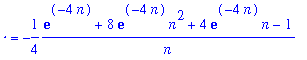
![V[n] = Int(n^2*x^2*exp(-2*n*x),x = 0 .. 2)](images/lab12170.gif)
| > |
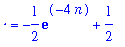
limit( value(V7), n=infinity );
|

Maple evaluates this integral:
![V[n] = -1/4*(exp(-4*n)+8*exp(-4*n)*n^2+4*exp(-4*n)*n-1)/n](images/lab12173.gif)
In the limit as
 increases towards infinity, the values of these integrals rapidly decay to zero.
| > |
DisplayPtSeq( V7, n=[1,2,4,8,16] );
|
![[Maple Plot]](images/lab12175.gif)
Example 8
For the final example, consider the sequence of functions on [0,2] defined to be
| > |
F8 := sqrt(n)*exp(-n*x):
f[n](x) = F8;
|
 = n^(1/2)*exp(-n*x)](images/lab12176.gif)
Initial Inspection
This sequence should be fairly simple to evaluate from a few appropriately selected plots.
| > |
AnimateFnSeq( F8, n=[1,2,4,8,16,32], x=0..2 );
|
![[Maple Plot]](images/lab12177.gif)

Pointwise Convergence
| > |
DisplayPtSeq( eval( F8-G8,x=1/2), n=[1,2,4,8,16,32] );
|
![[Maple Plot]](images/lab12179.gif)
Uniform Convergence
| > |
DisplayFnSeq( abs(F8-G8), n=[1,2,4,8,16,32], x=0..2 );
|
![[Maple Plot]](images/lab12180.gif)
Convergence in the Norm
| > |
V8 := Int( simplify(abs(F8-G8)^2), x=0..2 ):
V[n] = V8;
`` = value( V8 ) assuming posint;
|
![V[n] = Int(exp(-2*Re(n*x))*abs(n),x = 0 .. 2)](images/lab12181.gif)
| > |
DisplayPtSeq( V8, n=[1,2,4,8,16] );
|
![[Maple Plot]](images/lab12183.gif)
Lab Questions
1. [ 2 pts] Create a table [
Excel spreadsheet] that summarizes the results of each example considered above.
2. [5 pts] Based on your table in 1. decide if the following statements are true or false:
a. uniform convergence implies pointwise convergence
b. uniform convergence implies convergence in norm
c. pointwise convergence implies uniform convergence
d. pointwise convergence implies convergence in norm
e. convergence in norm implies uniform convergence
f. convergence in norm implies pointwise convergence
For each false statement, indicate one Example from earlier in the lab that supports your conclusion.
3. [2 pts] Integration problem. Show all steps in the evaluation of the integrals
V2a
=
 =
=
 in Example 2. You may use any technology to help solve this problem. Your answer, however, must explain all steps in the evaluation.